Art from code

Getting started

Code

library(tidyverse)
library(NatParksPalettes)
library(patchwork)
library(scales)
library(ggthemes)
library(rayshader)
library(ambient)
library(tictoc)
library(here)
library(ggforce)
library(deldir)
library(voronoise)
library(truchet)
library(sf)

Code

# function to save ggplot objects
save <- function(object, version, width, height) {
  filename <- paste0(deparse(substitute(object)), "_v", version, "_", today(), ".png")
  
  ggsave(filename = here::here("activities", "images", filename), 
         plot = object,
         width = width,
         height = height, 
         units = "in",
         dpi = 150)
}

Art is theft

Cars

Code

ggplot(data = mpg, aes(x = cty, y = hwy, color = year, fill = manufacturer)) +
  geom_point(size = 6, shape = 22) +
  scale_fill_manual(values = natparks.pals("Volcanoes", n = 15, type = "continuous")) +
  theme_void() +
  theme(legend.position = "none")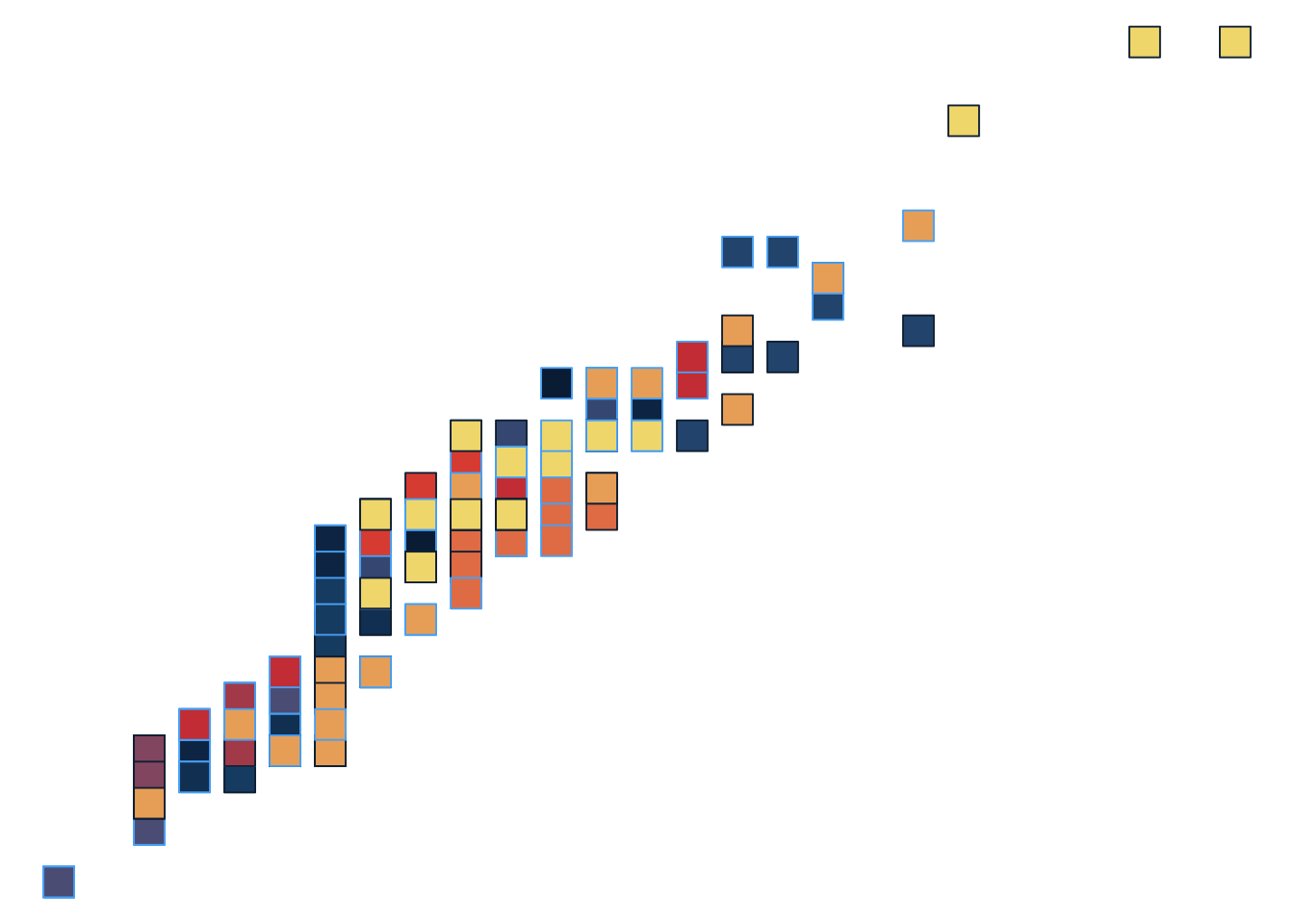

Technique

1. polar_art()

Function:

Code

polar_art <- function(seed, n, palette) {
  
  # set the state of the random number generator
  set.seed(seed)
  
  # data frame containing random values for 
  # aesthetics we might want to use in the art
  dat <- tibble(
    x0 = runif(n),
    y0 = runif(n),
    x1 = x0 + runif(n, min = -.2, max = .2),
    y1 = y0 + runif(n, min = -.2, max = .2),
    shade = runif(n), 
    size = runif(n)
  )
  
  # plot segments in various colours, using 
  # polar coordinates and a gradient palette
  dat |> 
    ggplot(aes(
      x = x0,
      y = y0,
      xend = x1,
      yend = y1,
      colour = shade,
      linewidth = size
    )) +
    geom_segment(show.legend = FALSE) +
    coord_polar() +
    scale_y_continuous(expand = c(0, 0)) +
    scale_x_continuous(expand = c(0, 0)) + 
    scale_colour_gradientn(colours = palette) + 
    scale_size(range = c(0, 10)) + 
    theme_void()
}

Output:

Code

polar_art(
  # change seed
  seed = 666, 
  # change numbers
  n = 200, 
  # change palette
  palette = c("cornflowerblue", "turquoise4", "orange", 
              "yellow", "darkgreen", "lavender")
)

2. polar_art_02()

Function:

Code

polar_art_02 <- function(seed, n, palette) {
  
  # set the state of the random number generator
  set.seed(seed)
  
  # data frame containing random values for 
  # aesthetics we might want to use in the art
  dat <- tibble(
    # changing distributions
    x0 = rnorm(n),
    y0 = rnbinom(n, size = rpois(1, 10), prob = 0.5),
    x1 = x0 + runif(n, min = -.2, max = .2),
    y1 = y0*2 + rbeta(n, shape1 = 3, shape2 = 2),
    shade = rnorm(n), 
    size = rpois(n, 20)
  )
  
  # plot segments in various colours, using 
  # polar coordinates and a gradient palette
  dat |> 
    ggplot(aes(
      x = x0,
      y = y0,
      xend = x1,
      yend = y1,
      colour = shade,
      linewidth = size
    )) +
    geom_segment(show.legend = FALSE) +
    coord_polar() +
    scale_y_continuous(expand = c(0, 0)) +
    scale_x_continuous(expand = c(0, 0)) + 
    scale_colour_gradientn(colours = palette) + 
    scale_size(range = c(0, 10)) + 
    theme_void()
}

Output:

Code

polarpalette <- c("cornflowerblue", "turquoise4", "orange", 
              "yellow", "darkgreen", "lavender")

polar50 <- polar_art_02(seed = 666, n = 50, palette = polarpalette)

polar100 <- polar_art_02(seed = 666, n = 100, palette = polarpalette)

polar300 <- polar_art_02(seed = 666, n = 300, palette = polarpalette)

polar50 + polar100 + polar300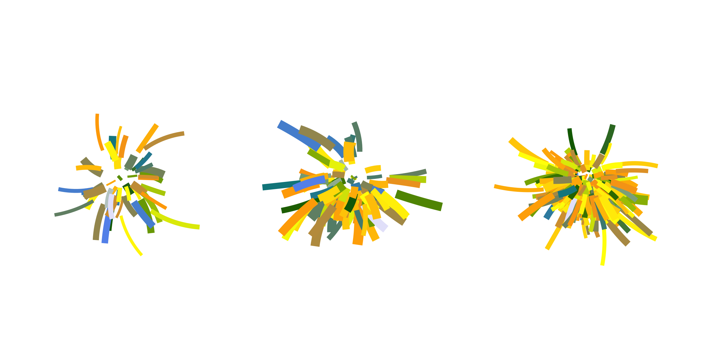

3. Versioning

It’s a “random” process - different output every time!

Color

1. sample_canva()

Function:

Code

# the original function from the first session
sample_canva <- function(seed = NULL) {
  if(!is.null(seed)) set.seed(seed)
  sample(ggthemes::canva_palettes, 1)[[1]]
}

# the extended function used in later sessions
sample_canva2 <- function(seed = NULL, n = 4) {
  if(!is.null(seed)) set.seed(seed)
  sample(ggthemes::canva_palettes, 1)[[1]] |>
    (\(x) colorRampPalette(x)(n))()  
}

Output:

Code

canva50 <- polar_art(seed = 666, n = 452, palette = sample_canva(seed = 50))
canva1000 <- polar_art(seed = 1, n = 323, palette = sample_canva(seed = 1000))
canva50000 <- polar_art(seed = 234987, n = 797, palette = sample_canva(seed = 50000))

canva50 + canva1000 + canva50000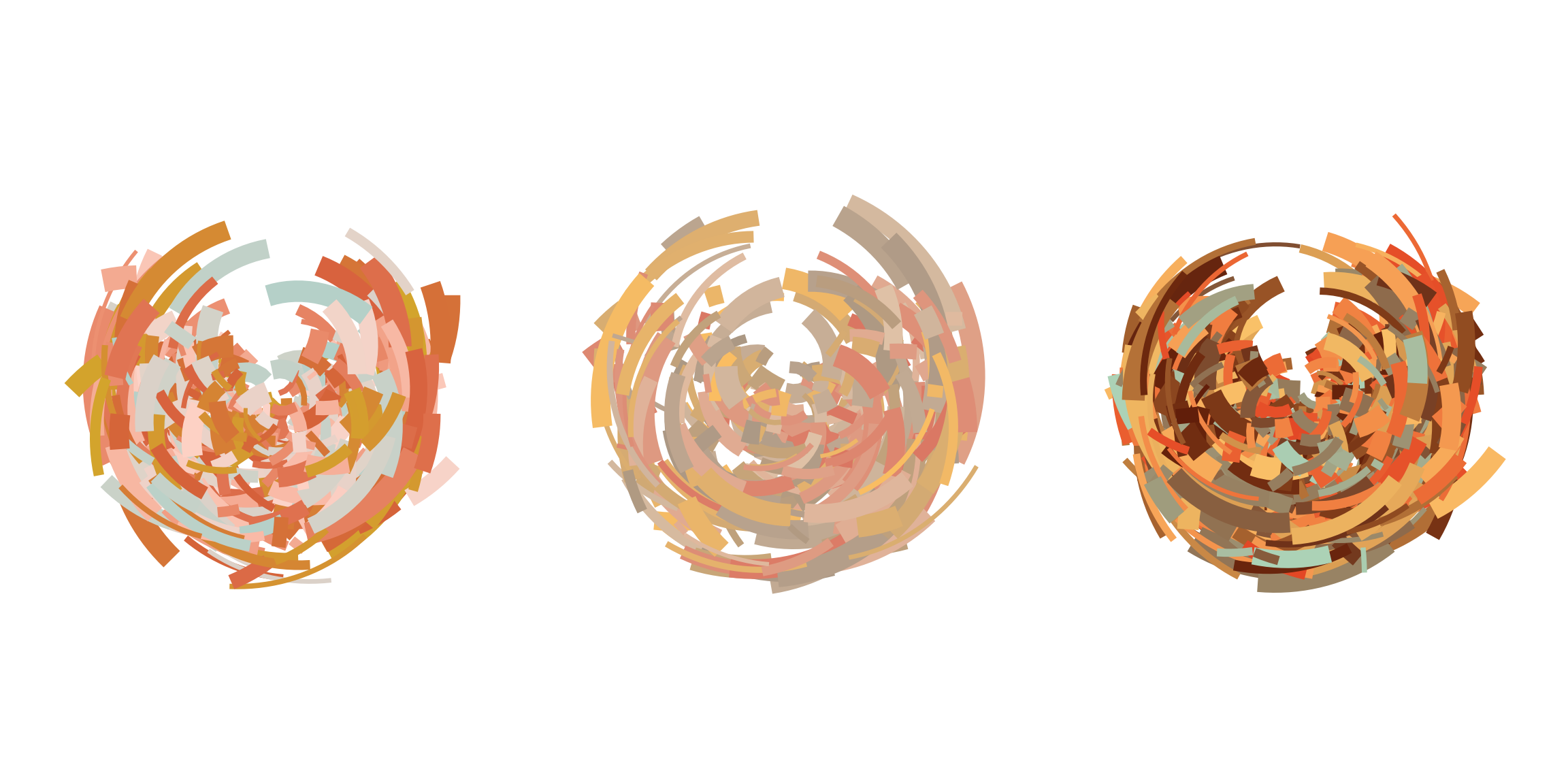

2. sample_named_colors()

Function:

Code

sample_named_colors <- function(n) {
  # sample from list of named colors in R
  sample(x = colours(distinct = TRUE), 
         size = n,
         replace = FALSE)
}

Output:

Code

sample1 <- polar_art(seed = 666, n = 50, palette = sample_named_colors(n = 50))
sample2 <- polar_art(seed = 111, n = 90, palette = sample_named_colors(n = 100))
sample3 <- polar_art(seed = 444, n = 150, palette = sample_named_colors(n = 10))

sample1 + sample2 + sample3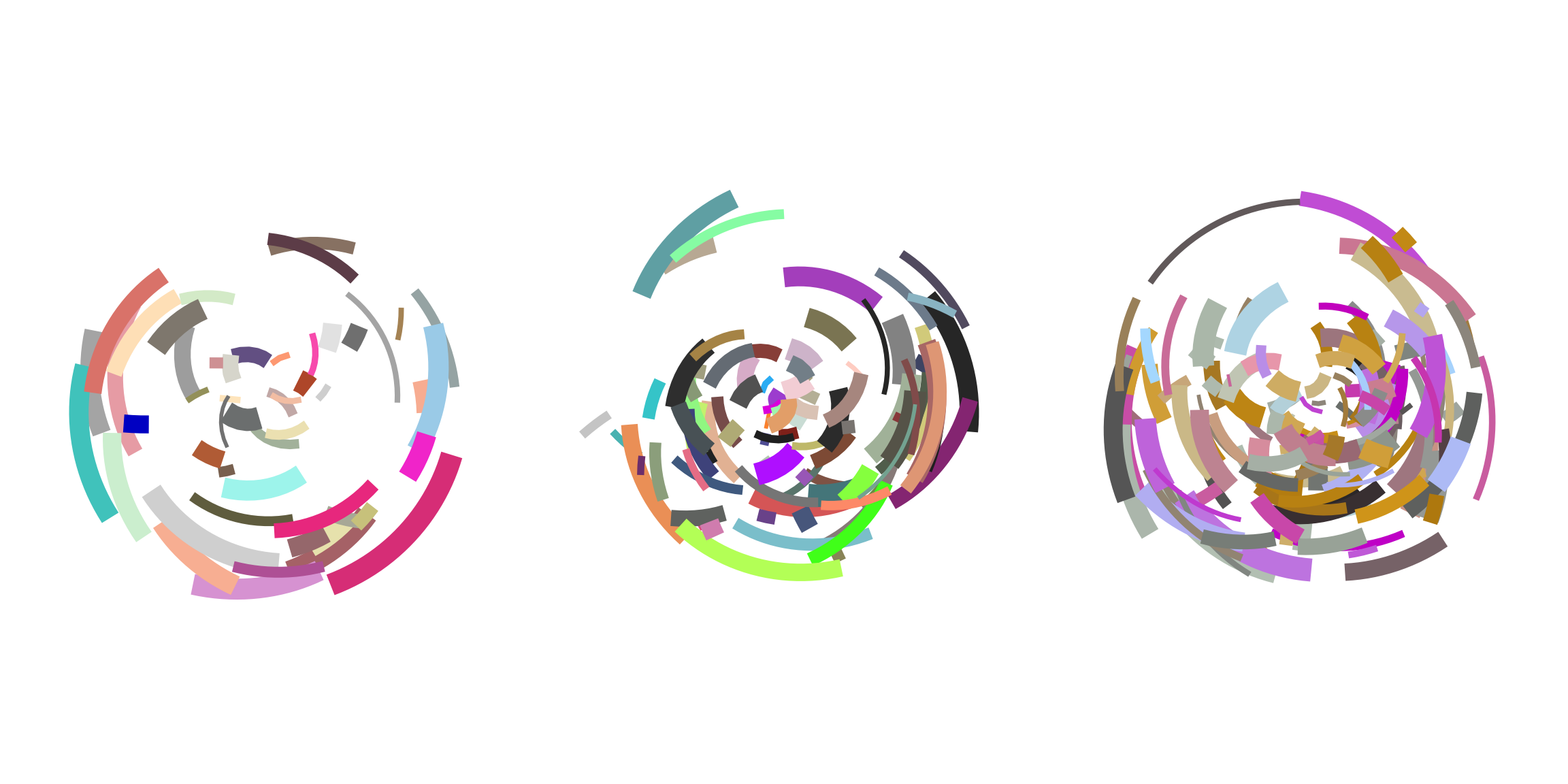

3. sample_canva_random()

Function:

Code

sample_canva_random <- function(seed = NULL) {
  # select a number of colors from a uniform distribution (and round)
  n <- round(runif(n = 1, min = 1, max = 600), digits = 0)
  
  # sample from list of all Canva colors
  sample(unlist(ggthemes::canva_palettes), 
         size = n,
         replace = FALSE)
}

Output:

Code

randomcanva1 <- polar_art(seed = 4245, n = 85, palette = sample_canva_random(seed = 1))
randomcanva2 <- polar_art(seed = 7832574, n = 425, palette = sample_canva_random(seed = 2))
randomcanva3 <- polar_art(seed = 453452, n = 254, palette = sample_canva_random(seed = 3))

randomcanva1 + randomcanva2 + randomcanva3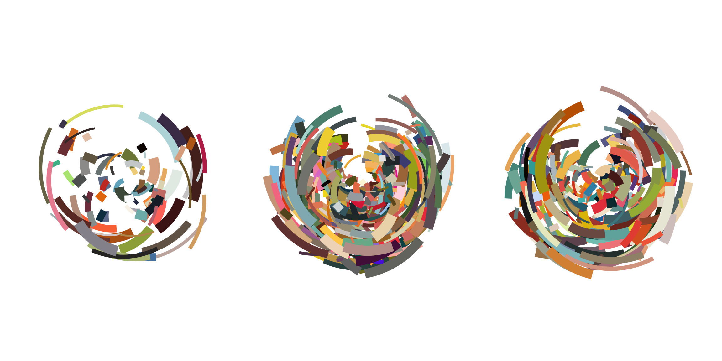

Composition

1. Function flexibility

Functions:

Code

sample_canva <- function(seed = NULL) {
  if(!is.null(seed)) set.seed(seed)
  sample(ggthemes::canva_palettes, 1)[[1]]
}

sample_data <- function(seed = NULL, n = 100){
  if(!is.null(seed)) set.seed(seed)
  dat <- tibble(
    x0 = runif(n),
    y0 = runif(n),
    x1 = x0 + runif(n, min = -.2, max = .2),
    y1 = y0 + runif(n, min = -.2, max = .2),
    shade = runif(n), 
    size = runif(n),
    shape = factor(sample(0:22, size = n, replace = TRUE))
  )
}

polar_styled_plot <- function(data = NULL, palette) {
  ggplot(
    data = data,
    mapping = aes(
      x = x0,
      y = y0,
      xend = x1,
      yend = y1,
      colour = shade,
      size = size
    )) + 
    coord_polar(clip = "off") +
    scale_y_continuous(
      expand = c(0, 0),
      limits = c(0, 1), 
      oob = scales::oob_keep
    ) +
    scale_x_continuous(
      expand = c(0, 0), 
      limits = c(0, 1), 
      oob = scales::oob_keep
    ) + 
    scale_colour_gradientn(colours = palette) + 
    scale_size(range = c(0, 10)) + 
    theme_void() + 
    guides(
      colour = guide_none(),
      size = guide_none(),
      fill = guide_none(),
      shape = guide_none()
    )
}

Output with modifications to sample data, using polar_styled_plot(), and using geoms:

Code

# changing seed
sampledat1 <- sample_data(n = 25, seed = 666) 

sampledat1plot <- polar_styled_plot(palette = sample_canva(seed = 100)) + 
  # using segment
  geom_segment(data = sampledat1, linetype = "331311") +
  # adding line
  geom_line(data = sampledat1) +
  # adding segment
  geom_segment(data = sampledat1, aes(x = x0, xend = x1), linewidth = 0.5)

# changing n
sampledat2 <- sample_data(n = 100, seed = 666) 

sampledat2plot <- polar_styled_plot(palette = sample_canva(seed = 44)) + 
  geom_point(data = sampledat2, aes(size = (y0 - y1)^2)) +
  # adding segment
  geom_segment(data = sampledat2, aes(y = y0, yend = y1), linewidth = 1) +
  geom_segment(data = sampledat2, aes(x = x0, xend = x0 + 0.11), alpha = 0.2)

sampledat1plot + sampledat2plot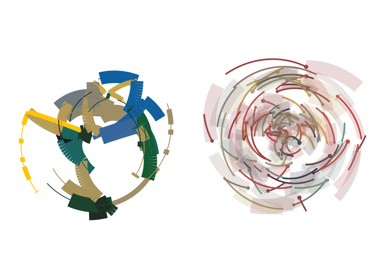

2. my_styled_plot()

Function:

Code

my_styled_plot <- function(data = NULL, palette) {
  ggplot(
    data = data,
    mapping = aes(
      x = x0,
      y = y0,
      xend = x1,
      yend = y1,
      colour = shade,
      size = size
    )) + 
    # coord_cartesian() +
    scale_y_continuous(
      expand = c(0, 0),
      limits = c(0, 1), 
      oob = scales::oob_keep
    ) +
    scale_x_continuous(
      expand = c(0, 0), 
      limits = c(0, 1), 
      oob = scales::oob_keep
    ) + 
    scale_colour_gradientn(colours = palette) + 
    scale_size(range = c(0, 10)) + 
    theme_void() + 
    guides(
      colour = guide_none(),
      size = guide_none(),
      fill = guide_none(),
      shape = guide_none()
    )
}

Output:

Code

sampledat3 <- sample_data(n = 100, seed = 666) 

msp1 <- my_styled_plot(data = sampledat3, palette = sample_canva_random(seed = 40)) +
  geom_line()

msp2 <- my_styled_plot(data = sampledat3, palette = sample_canva_random(seed = 40)) +
  geom_segment(aes(x = 0, xend = x1, y = 0, yend = y1), linewidth = 1) +
  coord_polar()

msp3 <- my_styled_plot(data = sampledat3, palette = sample_canva_random(seed = 40)) +
  geom_point() +
  coord_polar()

msp1 + msp2 + msp3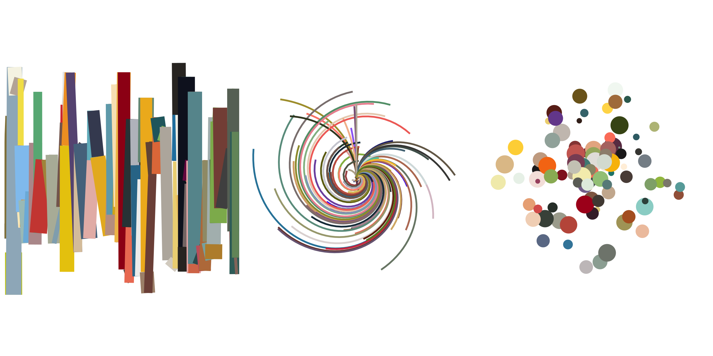

Shading tricks

Rayshader art

Circles

Functions:

Code

# input: coordinates, center, radius
# output: logical TRUE whenever coordinates fall within circle defined by radius
is_within_circle <- function(x_coord, y_coord, x_center, y_center, radius) {
  (x_coord - x_center)^2 + (y_coord - y_center)^2 < radius^2
}

# generates n circles at random
# output: long grid with x, y, and paint
# paint is the proportion of circles that each point falls in
additive_circles <- function(n = 5, pixels = 1000, seed = NULL) {
  
  if(!is.null(seed)) set.seed(seed)
  
  # setup canvas
  art <- long_grid(
    x = seq(0, 1, length.out = pixels),
    y = seq(0, 1, length.out = pixels)
  )
  art$paint <- 0
  
  for(i in 1:n) {
    
    # sample a random circle
    x_center <- runif(1, min = .3, max = .7)
    y_center <- runif(1, min = .3, max = .7)
    radius <- runif(1, min = .05, max = .25)
    
    # add +1 to all points inside the circle
    art <- art |>
      mutate(
        paint = paint + is_within_circle(
          x, y, x_center, y_center, radius
        )
      )
  }
  
  # normalise paint to [0, 1] range and return
  art$paint <- normalise(art$paint)
  return(art)
}

Generate tibble and array:

Code

circle_art <- additive_circles(seed = 666) 

circle_array <- circle_art |>
  as.array(value = paint) 

Output:

Code

# use ggplot
ggplot(circle_art, aes(x = x, y = y, fill = as.factor(paint))) +
  geom_raster(show.legend = FALSE) +
  scale_fill_manual(values = natparks.pals("GrandCanyon", n = 4, type = "continuous")) +
  theme_void() +
  coord_cartesian()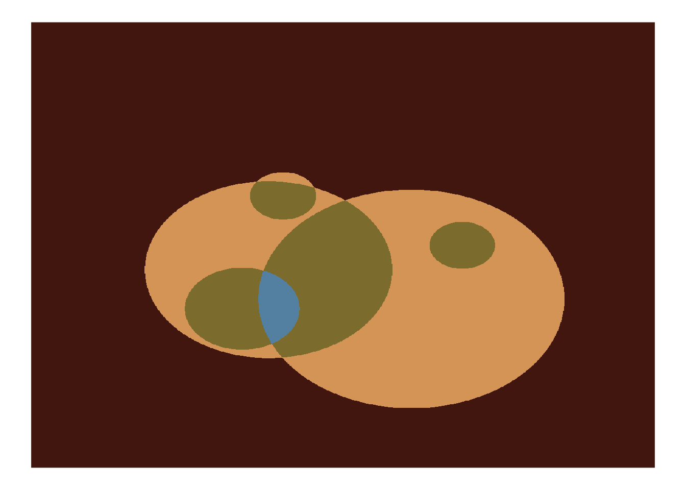

Code

# plot as raster
circle_array %>% 
  raster::image(axes = FALSE, asp = 1, useRaster = TRUE)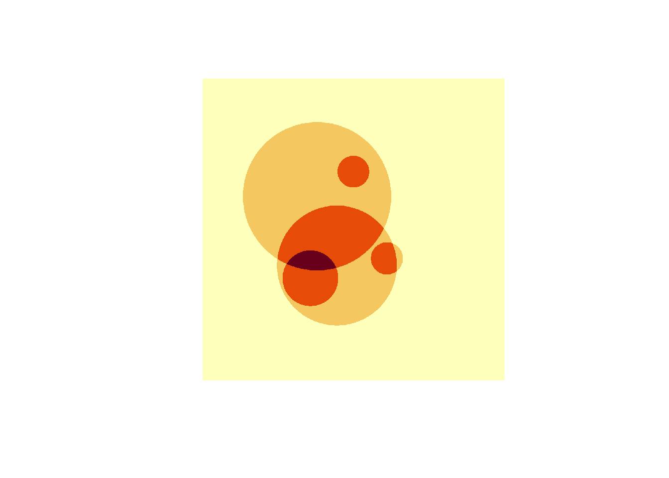

Shadows

Code

circle_shadow1 <- ray_shade(
  heightmap = circle_array,
  sunaltitude = 15, 
  sunangle = 135,
  zscale = .01,
  multicore = TRUE
)

circle_scape1 <- circle_array |> 
  height_shade() |>
  add_shadow(
    shadowmap = circle_shadow1,
    max_darken = .1
  )

circle_shadow2 <- ray_shade(
  heightmap = circle_array,
  sunaltitude = 20, 
  sunangle = 170,
  zscale = 0.1,
  multicore = TRUE
)

circle_scape2 <- circle_array |> 
  height_shade() |>
  add_shadow(
    shadowmap = circle_shadow2,
    max_darken = .1
  )

tic()
plot_map(circle_scape1, rotate = 270)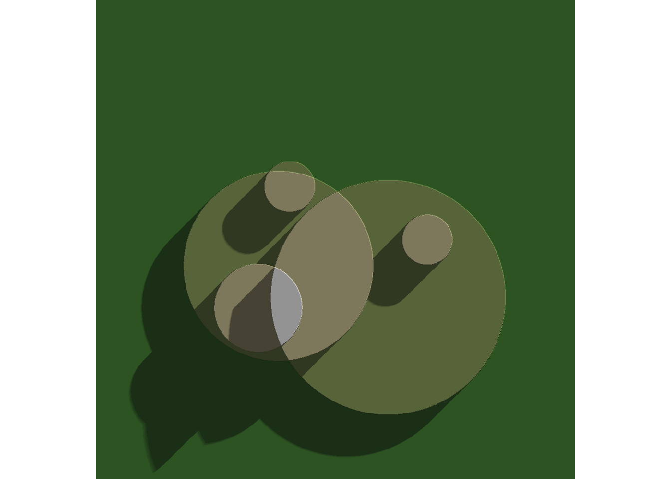

Code

plot_map(circle_scape2, rotate = 180)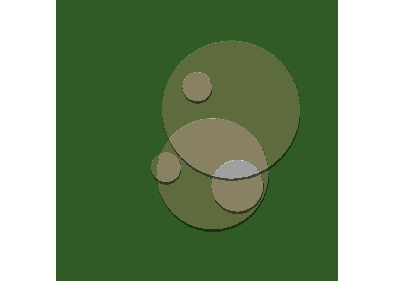

Code

toc()

1.373 sec elapsed

Shadowed noise fields

shaded_ridge_art()

Function:

Code

ridge_art <- function(seed = NULL, pixels = 2000) {
  
  if(!is.null(seed)) set.seed(seed)
  long_grid(
    x = seq(from = 0, to = 1, length.out = pixels),
    y = seq(from = 0, to = 1, length.out = pixels)
  ) |> 
    mutate(
      paint = fracture(
        x = x, 
        y = y,
        noise = gen_simplex,
        fractal = ridged,
        octaves = 8,
        frequency = 10,
        seed = seed
      ),
      paint = normalise(paint)
    ) |>
    as.array(value = paint)
}

shaded_ridge_art <- function(seed = NULL) {
  
  art <- ridge_art(seed) 
  height_shade(
    heightmap = art,
    texture = sample_canva2(seed, 256)
  ) |>
    add_shadow(
      shadowmap = ray_shade(
        heightmap = art, 
        sunaltitude = 30, 
        sunangle = 90,
        multicore = TRUE, 
        zscale = .05
      ), 
      max_darken = .1
    ) |>
    plot_map()
}

New functions:

Code

ridge_art_02 <- function(seed = NULL, pixels = 2000) {
  
  if(!is.null(seed)) set.seed(seed)
  long_grid(
    x = seq(from = 0, to = 1, length.out = pixels),
    y = seq(from = 0, to = 1, length.out = pixels)
  ) |> 
    mutate(
      paint = fracture(
        x = x, 
        y = y,
        noise = gen_simplex,
        fractal = ridged,
        octaves = 8,
        frequency = 10,
        seed = seed
      ),
      paint = normalise(paint)
    ) |>
    as.array(value = paint)
}

shaded_ridge_art_02 <- function(seed = NULL) {
  
  art <- ridge_art_02(seed) 
  height_shade(
    heightmap = art,
    texture = sample_named_colors(4)
  ) |>
    add_shadow(
      shadowmap = ray_shade(
        heightmap = art, 
        sunaltitude = 30, 
        sunangle = 90,
        multicore = TRUE, 
        zscale = .05
      ), 
      max_darken = .1
    ) |>
    plot_map()
}

Output:

Code

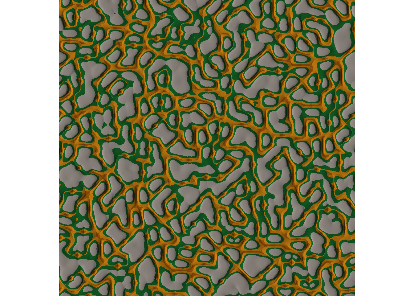
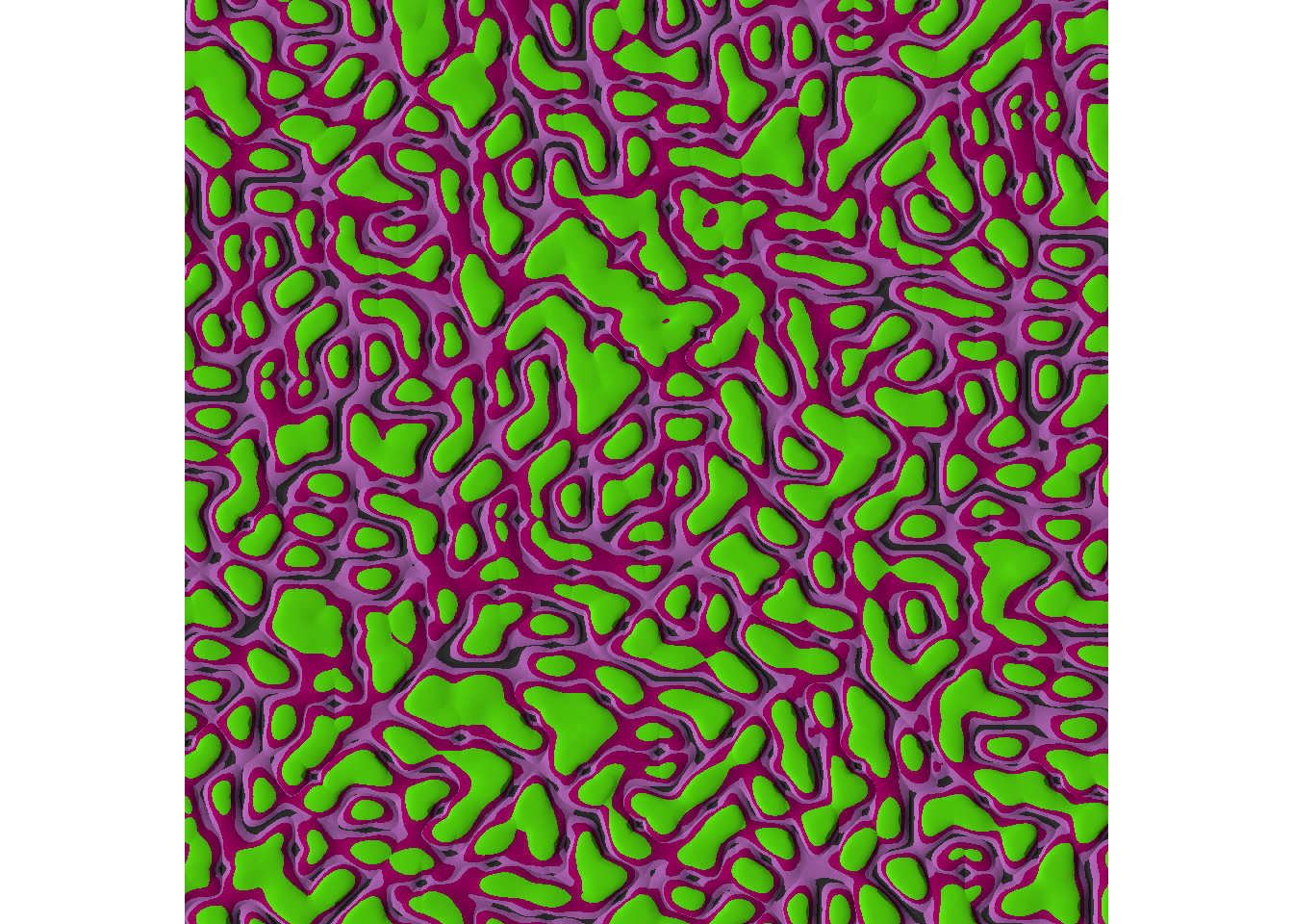
shaded_ridge_art_02(1)
shaded_ridge_art_02(10)
shaded_ridge_art_02(100)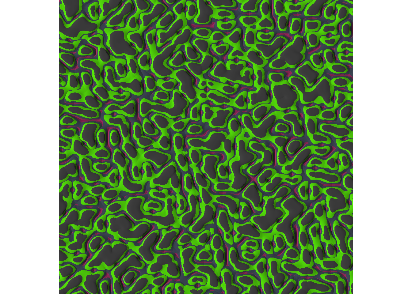

Fractured terrain

Functions:

Code

transform_to_curl_space <- function(x, y, frequency = 1, octaves = 10) {
  curl_noise(
    generator = fracture,
    noise = gen_simplex,
    fractal = fbm,
    octaves = octaves,
    frequency = frequency,
    x = x,
    y = y
  )
}


define_worley_cells <- function(x, y, frequency = 3, octaves = 6) {
  fracture(
    noise = gen_worley,
    fractal = billow,
    octaves = octaves,
    frequency = frequency,
    value = "cell",
    x = x,
    y = y
  ) |>
    rank() |> 
    normalise()
}


simplex_noise <- function(x, y, frequency = .1, octaves = 10) {
  fracture(
    noise = gen_simplex,
    fractal = ridged,
    octaves = octaves,
    frequency = frequency,
    x = x,
    y = y
  ) |>
    normalise()
}


ice_floe <- function(seed) {
  
  set.seed(seed)
  
  grid <- long_grid(
    x = seq(0, 1, length.out = 2000),
    y = seq(0, 1, length.out = 2000)
  )
  
  coords <- transform_to_curl_space(grid$x, grid$y)
  
  grid |>
    mutate(
      cells = define_worley_cells(coords$x, coords$y),
      paint = simplex_noise(x + cells, y + cells),
      paint = normalise(paint)
    ) |>
    as.array(value = paint)
}

shaded_ice_floe <- function(seed) {
  
  art <- ice_floe(seed)
  
  height_shade(
    heightmap = art,
    texture = sample_canva2(seed, 256)
  ) |>
    add_shadow(
      shadowmap = ray_shade(
        heightmap = art, 
        sunaltitude = 30, 
        sunangle = 90,
        multicore = TRUE, 
        zscale = .005
      ), 
      max_darken = .05
    ) |>
    plot_map()
}

Output:

Code

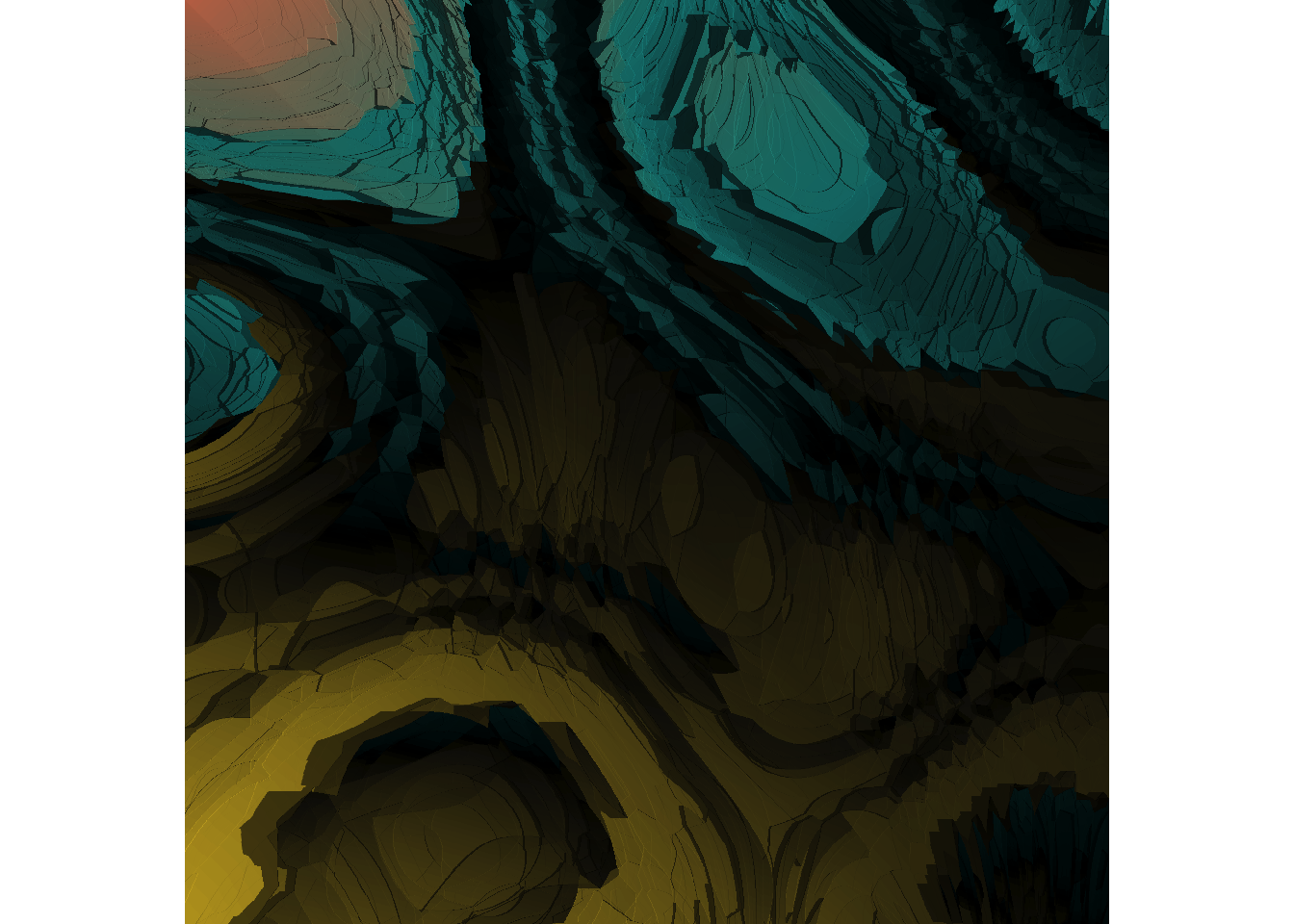
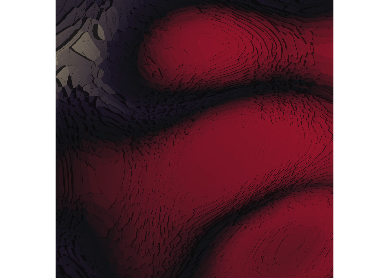
tic()
shade_1 <- shaded_ice_floe(111)
shade_2 <- shaded_ice_floe(222)
shade_3 <- shaded_ice_floe(333)
toc()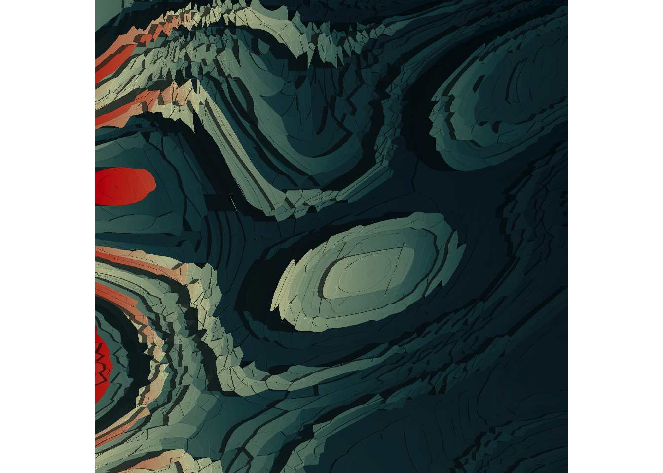

47.825 sec elapsed

Icescape script:

Code

icescape_3d <- function(seed) {
  
  ice_height <- matrix(0, 2500, 2500)
  ice_height[251:2250, 251:2250] <- ice_floe(seed)
  
  ice_scape <- height_shade(
    heightmap = ice_height,
    texture = sample_canva2(seed, 256)
  ) |>
    add_shadow(
      shadowmap = ray_shade(
        heightmap = ice_height, 
        sunaltitude = 30, 
        sunangle = 90,
        multicore = TRUE, 
        zscale = .005
      ), 
      max_darken = .05
    )
  
  plot_3d(
    hillshade = ice_scape,
    heightmap = ice_height,
    theta = 45,
    phi = 30,
    zoom = .75,
    zscale = .001,
    background = "#222222",
    shadow = FALSE,
    soliddepth = .5,
    solidcolor = "#222222",
    windowsize = c(2500, 1500)
  )
  
  render_snapshot(
    filename = here("activities", "images", paste0("icescape_3d_", seed, "_", today(), ".png")), 
    clear = TRUE
  )
}

tic()
icescape_3d(444)
toc()

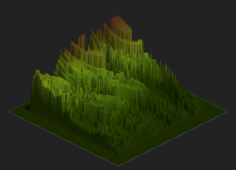
note about the icescape

This took a while to run, so I just ran it, saved the output as in the function, and am embedding the image here.

Tiles and tesselations

Rectangle subdivision

Functions:

Code

# blocks: each row is a block, column is the area of that block
# choose_rectangle randomly selects row with probability proportional to the area
# larger blocks are more likely to be chosen
choose_rectangle <- function(blocks) {
  sample(nrow(blocks), 1, prob = blocks$area)
}

# decides where the break in the subdivision will be
choose_break <- function(lower, upper) {
  round((upper - lower) * runif(1))
}

# creates a tibble with characteristics that define the rectangle
create_rectangles <- function(left, right, bottom, top, value) {
  tibble(
    left = left,
    right = right,
    bottom = bottom,
    top = top,
    width = right - left,
    height = top - bottom,
    area = width * height,
    value = value
  )
}

# takes a rectangle object from create_rectangles
# breaks from choose_break
# creates two new rectangles that replace the old one
split_rectangle_x <- function(rectangle, new_value) {
  with(rectangle, {
    split <- choose_break(left, right)
    new_left  <- c(left, left + split)
    new_right <- c(left + split, right)
    new_value <- c(value, new_value)
    create_rectangles(new_left, new_right, bottom, top, new_value)
  })
}

# same as above
split_rectangle_y <- function(rectangle, new_value) {
  with(rectangle, {
    split <- choose_break(bottom, top)
    new_bottom <- c(bottom, bottom + split)
    new_top <- c(bottom + split, top)
    new_value <- c(value, new_value)
    create_rectangles(left, right, new_bottom, new_top, new_value)
  })
}

# random decision to split vertically or horizontally
split_rectangle <- function(rectangle, value) {
  if(runif(1) < .5) {
    return(split_rectangle_x(rectangle, value))
  }
  split_rectangle_y(rectangle, value)
}

# takes "block", selects one rectangle to be subdivided, then splits
split_block <- function(blocks, value) {
  old <- choose_rectangle(blocks) 
  new <- split_rectangle(blocks[old, ], value)
  bind_rows(blocks[-old, ], new)
}

# apply split_block a bunch of times
subdivision <- function(ncol = 1000, 
                        nrow = 1000, 
                        nsplits = 50, 
                        seed = NULL) {
  
  if(!is.null(seed)) set.seed(seed)
  blocks <- create_rectangles(
    left = 1, 
    right = ncol, 
    bottom = 1, 
    top = nrow, 
    value = 0
  )
  reduce(1:nsplits, split_block, .init = blocks)
}

# plots the rectangles
develop <- function(div, seed = NULL) {
  
  div |> 
    ggplot(aes(
      xmin = left, 
      xmax = right, 
      ymin = bottom, 
      ymax = top,
      fill = value
    )) +
    geom_rect(
      colour = "#ffffff", 
      size = 3,
      show.legend = FALSE
    ) +
    scale_fill_gradientn(
      colours = sample_canva2(seed)
    ) +
    coord_equal() +
    theme_void()
}

Code

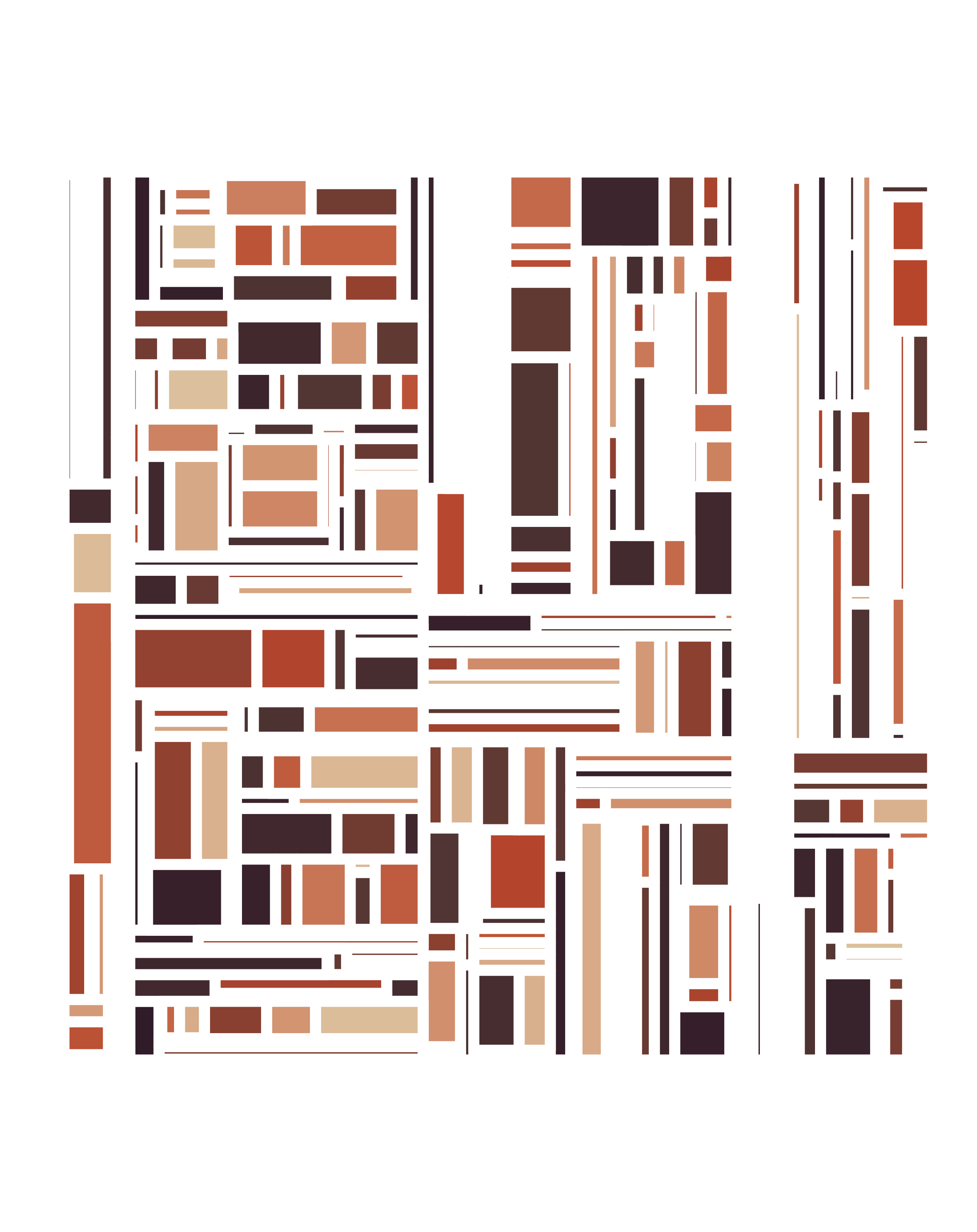
pic1 <- subdivision(nsplits = 20, seed = 2) %>% 
  develop() 

pic2 <- subdivision(nsplits = 50, seed = 666) %>% 
  develop() 

pic3 <- subdivision(nsplits = 500, seed = 10) %>% 
  develop() 

save(pic1)
save(pic2)
save(pic3)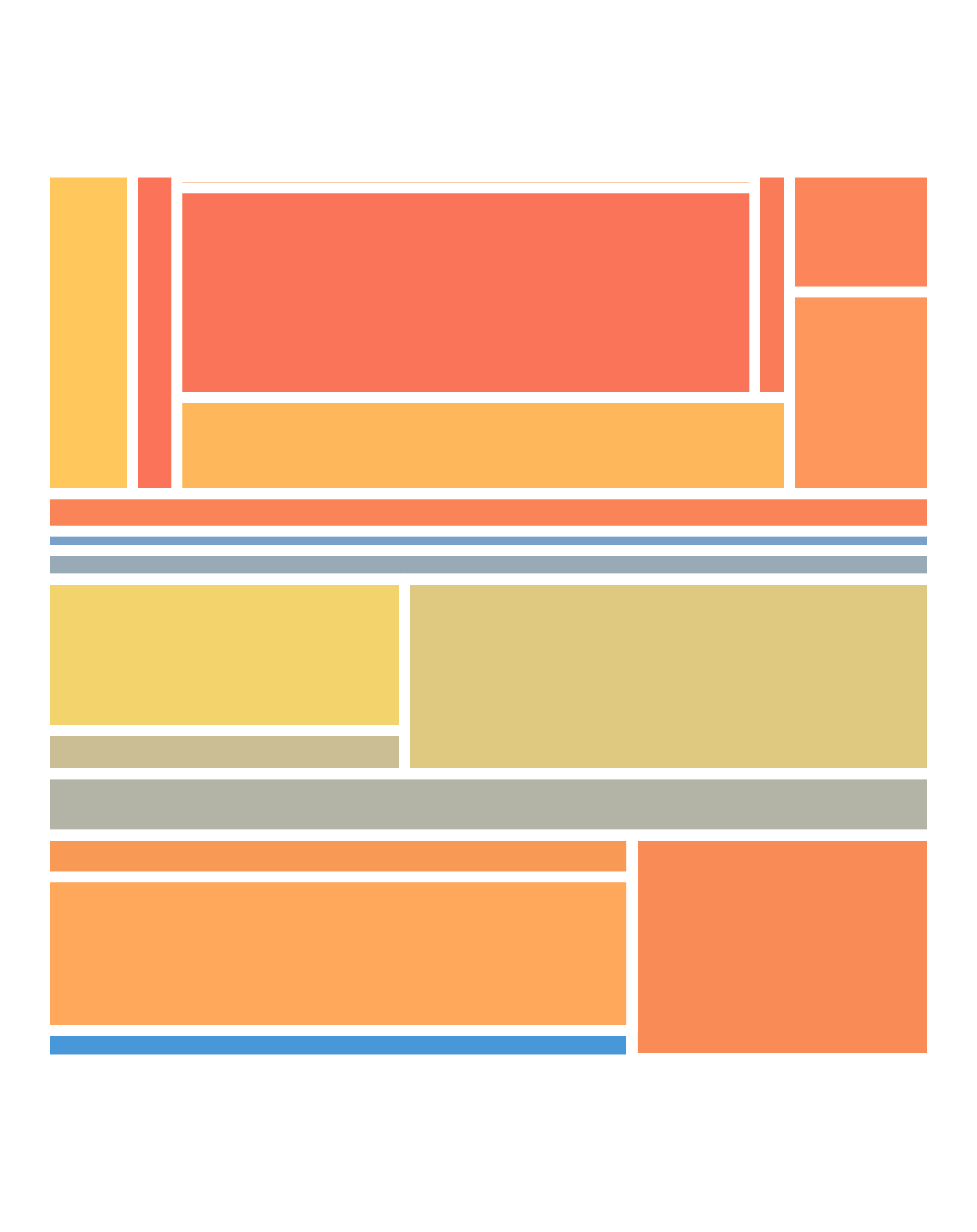

Mosaica

Functions:

Code

# input: rectangle
# divides rectanlge into grid with squares with length 1
# assigns squares some fill value from a randomly sampled fractal
fill_rectangle <- function(left, right, bottom, top, width, 
                           height, area, value, nshades = 100) {
  
  set.seed(value)
  fractals <- list(billow, fbm, ridged)
  generators <- list(gen_simplex, gen_perlin, gen_worley)
  
  expand_grid(
    x = left:right, 
    y = bottom:top, 
  ) |>
    mutate(
      fill = 10 * value + fracture(
        x = x * sample(-3:3, 1),
        y = y * sample(-3:3, 1),
        noise = sample(generators, 1)[[1]],
        fractal = sample(fractals, 1)[[1]],
        octaves = sample(10, 1),
        frequency = sample(10, 1) / 20,
        value = "distance2"
      ) |>
        normalise(to = c(1, nshades)) |> 
        round()
    )
}

# plot using ggplot/geom_tile
draw_mosaic <- function(dat, palette) {
  background <- sample(palette, 1)
  dat |>
    ggplot(aes(x, y, fill = fill)) +
    geom_tile(show.legend = FALSE, colour = background, size = .2) +
    scale_size_identity() +
    scale_colour_gradientn(colours = palette) +
    scale_fill_gradientn(colours = palette) +
    scale_x_continuous(expand = expansion(add = 5)) +
    scale_y_continuous(expand = expansion(add = 5)) +
    coord_equal() +
    theme_void() +
    theme(plot.background = element_rect(fill = background)) 
}

# actually does the generation and the drawing
mosaica <- function(ncol = 60, 
                    nrow = 60, 
                    nsplits = 30, 
                    seed = NULL) {
  
  subdivision(ncol, nrow, nsplits, seed) |>
    pmap_dfr(fill_rectangle) |> 
    slice_sample(prop = .995) |>
    filter(!is.na(fill)) |>
    draw_mosaic(palette = sample_canva2(seed))
}

Output:

Code

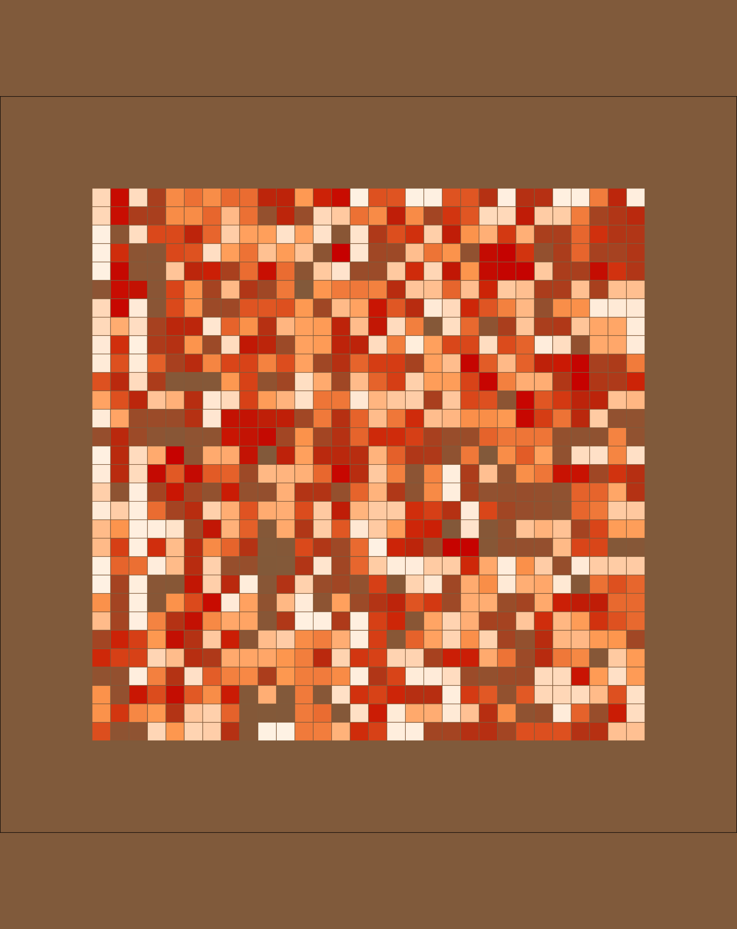
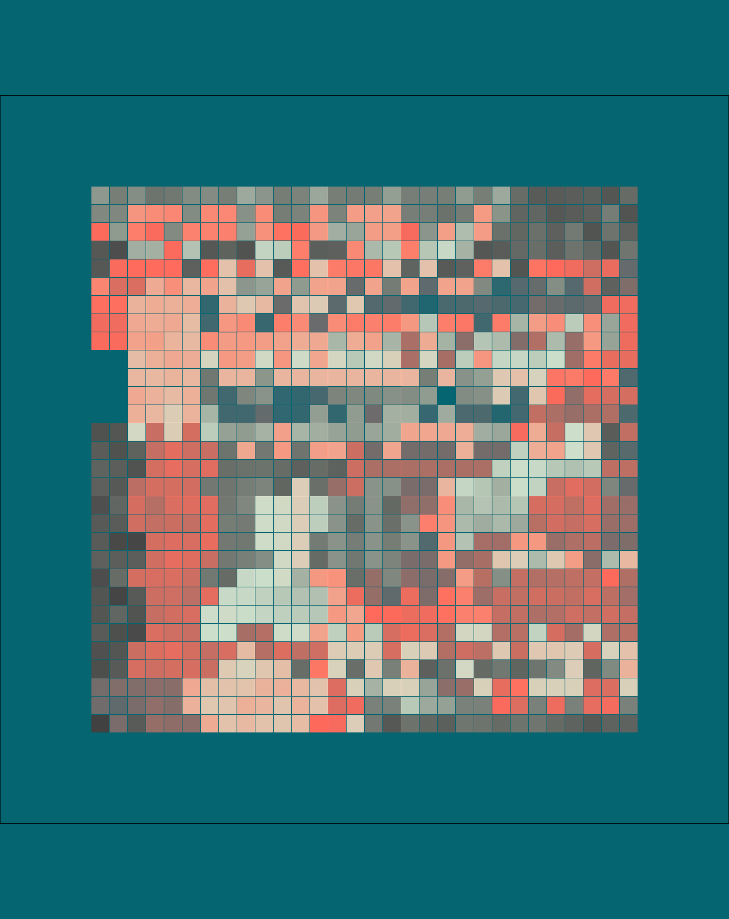
mosaic1 <- mosaica(ncol = 30, nrow = 30, nsplits = 300, seed = 666)
mosaic2 <- mosaica(ncol = 30, nrow = 30, nsplits = 1000, seed = 243)
mosaic3 <- mosaica(ncol = 30, nrow = 30, nsplits = 100, seed = 234098)

save(mosaic1)
save(mosaic2)
save(mosaic3)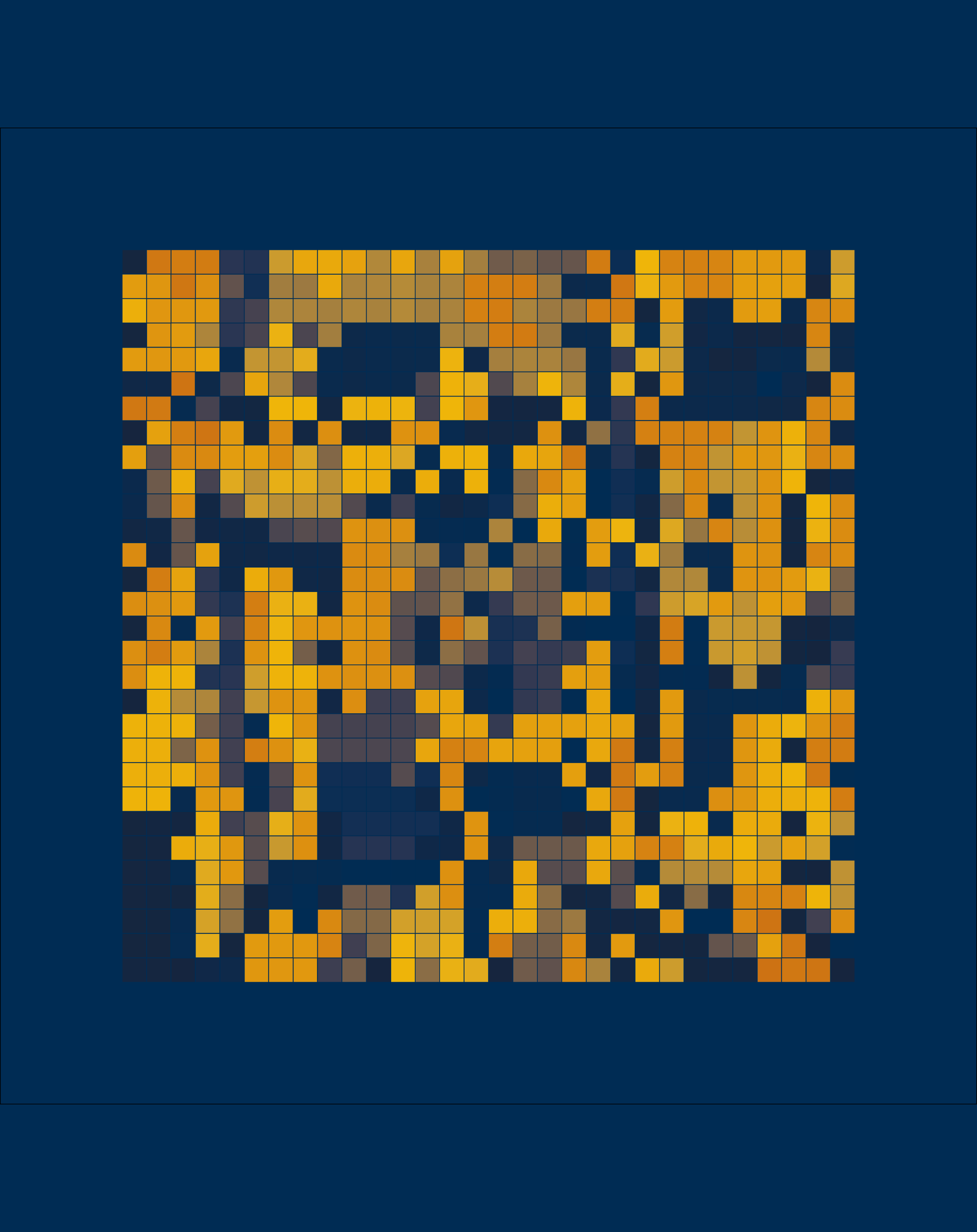

Voronoi tesselation

Example:

Code

set.seed(61)

dat <- tibble(
  x = runif(20),
  y = runif(20),
  val = runif(20)
)

bg_dat <- tibble(
  x = runif(500, min = -.5, max = 1.5),
  y = runif(500, min = -.5, max = 1.5)
)

pic <- ggplot(dat, aes(x, y, fill = val)) +
  coord_equal(xlim = c(-.3, 1.3), ylim = c(-.3, 1.3)) +
  guides(fill = guide_none()) +
  theme_void() + 
  theme(panel.background = element_rect(
    fill = "#222222", colour = "#222222"
  ))

pic2 <- pic + 
  geom_voronoi_tile(
    data = bg_dat,
    fill = "#333333", 
    radius = .01,
    expand = -.0025
  ) +
  geom_voronoi_tile(
    colour = "white", 
    max.radius = .2, 
    radius = .02,
    expand = -.005
  )

plot(pic2)

Playing around:

Code

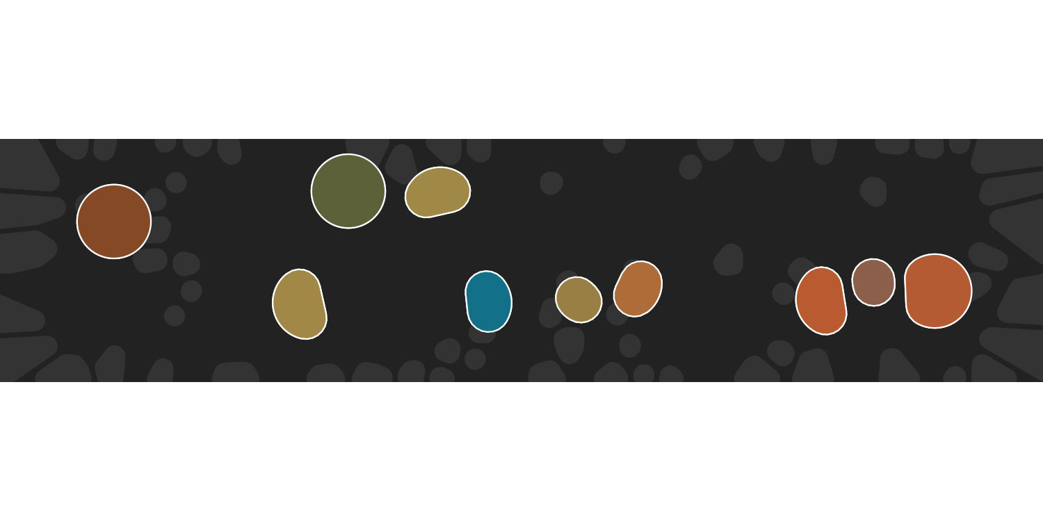
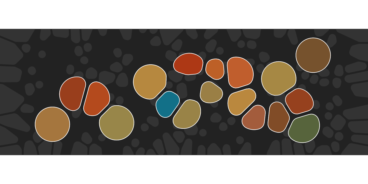
set.seed(10)

# voronoi data
dat2 <- tibble(
  # changing distributions
  x = rnorm(n = 20),
  y = rbeta(n = 20, shape1 = 1, shape2 = 3),
  val = runif(20)
)

# background tiles
bg_dat2 <- tibble(
  # liked these, so keeping them
  # make the min and max the coordinate limits
  x = runif(500, min = -2, max = 1.5),
  y = runif(500, min = -0.2, max = 1)
)

pic_sag <- ggplot(data = dat2, aes(x, y, fill = val)) +
  coord_equal(xlim = c(-2, 1.5), ylim = c(-0.2, 1)) +
  guides(fill = guide_none()) +
  theme_void() + 
  theme(panel.background = element_rect(
    fill = "#222222", colour = "#222222"
  )) +
  geom_voronoi_tile(aes(fill = val), color = "#FFFFFF", 
                    # makes them round
                    max.radius = 0.2, 
                    # rounds the corners
                    radius = 0.02,
                    # adds a little space
                    expand = -0.005) +
  scale_fill_gradientn(colors = natparks.pals("Saguaro", n = 20, type = "continuous"))

pic_sag

pic_sag_bg <- pic_sag + 
  geom_voronoi_tile(
    data = bg_dat2,
    fill = "#333333", 
    radius = .01,
    expand = -.0025
  ) +
  geom_voronoi_tile(
    colour = "white", 
    max.radius = .2, 
    radius = .02,
    expand = -.005
  )

pic_sag_bg

save(pic_sag_bg, version = "03", width = 10, height = 5)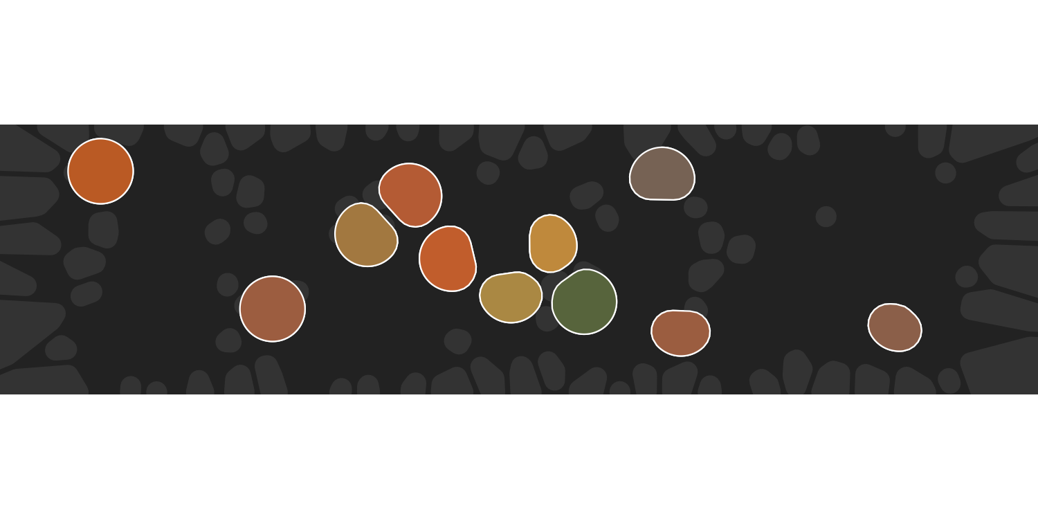

Studies in Voronoi baroque: Part I

Functions:

Code

unboxy <- function(iterations, layers) {
  
  coeffs <- array(
    data = runif(9 * layers, min = -1, max = 1), 
    dim = c(3, 3, layers)
  )
  
  point0 <- matrix(
    data = runif(3, min = -1, max = 1), 
    nrow = 1,
    ncol = 3
  )
  
  funs <- list(
    function(point) point + (sum(point ^ 2)) ^ (1/3),
    function(point) sin(point),
    function(point) 2 * sin(point)
  )
  
  update <- function(point, t) {
    l <- sample(layers, 1)
    f <- sample(funs, 1)[[1]]
    z <- point[3]
    point[3] <- 1
    point <- f(point %*% coeffs[,,l])
    point[3] <- (point[3] + z)/2
    return(point)
  }
  
  points <- accumulate(1:iterations, update, .init = point0)
  points <- matrix(unlist(points), ncol = 3, byrow = TRUE)
  points <- as_tibble(as.data.frame(points)) 
  names(points) <- c("x", "y", "val")
  return(points)
}

Output:

Code

# new data generation
set.seed(666)
unboxy_dat <- unboxy(iterations = 1000, layers = 5) 

ggplot(unboxy_dat, aes(x, y)) + 
  geom_point(colour = "white", show.legend = FALSE) +
  # new x and y limits
  # coord_equal(xlim = c(-2, 2), ylim = c(-2, 2)) + 
  # theme_void() +
  theme(panel.background = element_rect(
    fill = "#222222", colour = "#222222"
  ))

unboxy_pic1 <- ggplot(unboxy_dat, aes(x, y, fill = val)) +
  theme_void() + 
  coord_equal(xlim = c(-2, 0), ylim = c(-2, 0)) +
  scale_fill_gradientn(colours = natparks.pals("Olympic", n = 10, type = "continuous")) + 
  scale_x_continuous(expand = c(0, 0)) +
  scale_y_continuous(expand = c(0, 0)) +
  geom_voronoi_tile(
    colour = "#222222",
    linewidth = .2, 
    max.radius = 0.08,
    radius = 0.01,
    expand = -0.005,
    size = 0.2, 
    show.legend = FALSE
  )

unboxy_pic2 <- ggplot(unboxy_dat, aes(x, y, fill = val)) +
  theme_void() + 
  coord_equal(xlim = c(0, 2), ylim = c(-2, 0)) +
  scale_fill_gradientn(colours = natparks.pals("KingsCanyon", n = 10, type = "continuous")) + 
  scale_x_continuous(expand = c(0, 0)) +
  scale_y_continuous(expand = c(0, 0)) +
  geom_voronoi_tile(
    colour = "#222222",
    linewidth = .2, 
    max.radius = 0.08,
    radius = 0.01,
    expand = -0.005,
    size = 0.2, 
    show.legend = FALSE
  )

unboxy_pic3 <- ggplot(unboxy_dat, aes(x, y, fill = val)) +
  theme_void() + 
  coord_equal(xlim = c(0, 2), ylim = c(0, 2)) +
  scale_fill_gradientn(colours = natparks.pals("Everglades", n = 10, type = "continuous")) + 
  scale_x_continuous(expand = c(0, 0)) +
  scale_y_continuous(expand = c(0, 0)) +
  geom_voronoi_tile(
    colour = "#222222",
    linewidth = .2, 
    max.radius = 0.08,
    radius = 0.01,
    expand = -0.005,
    size = 0.2, 
    show.legend = FALSE
  )

save(object = unboxy_pic1, version = "02", width = 4, height = 4)

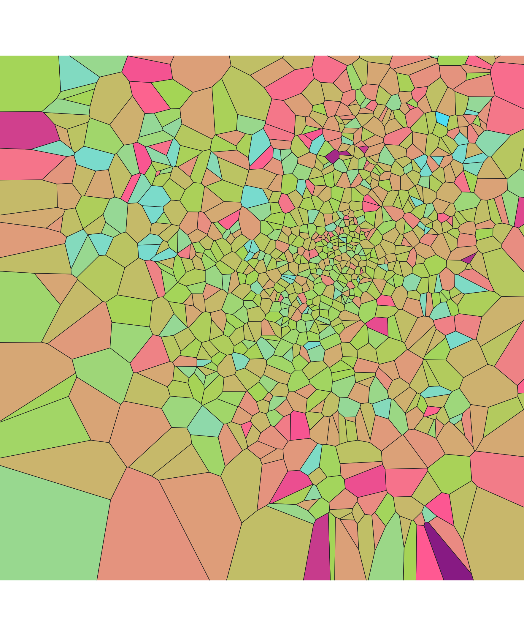
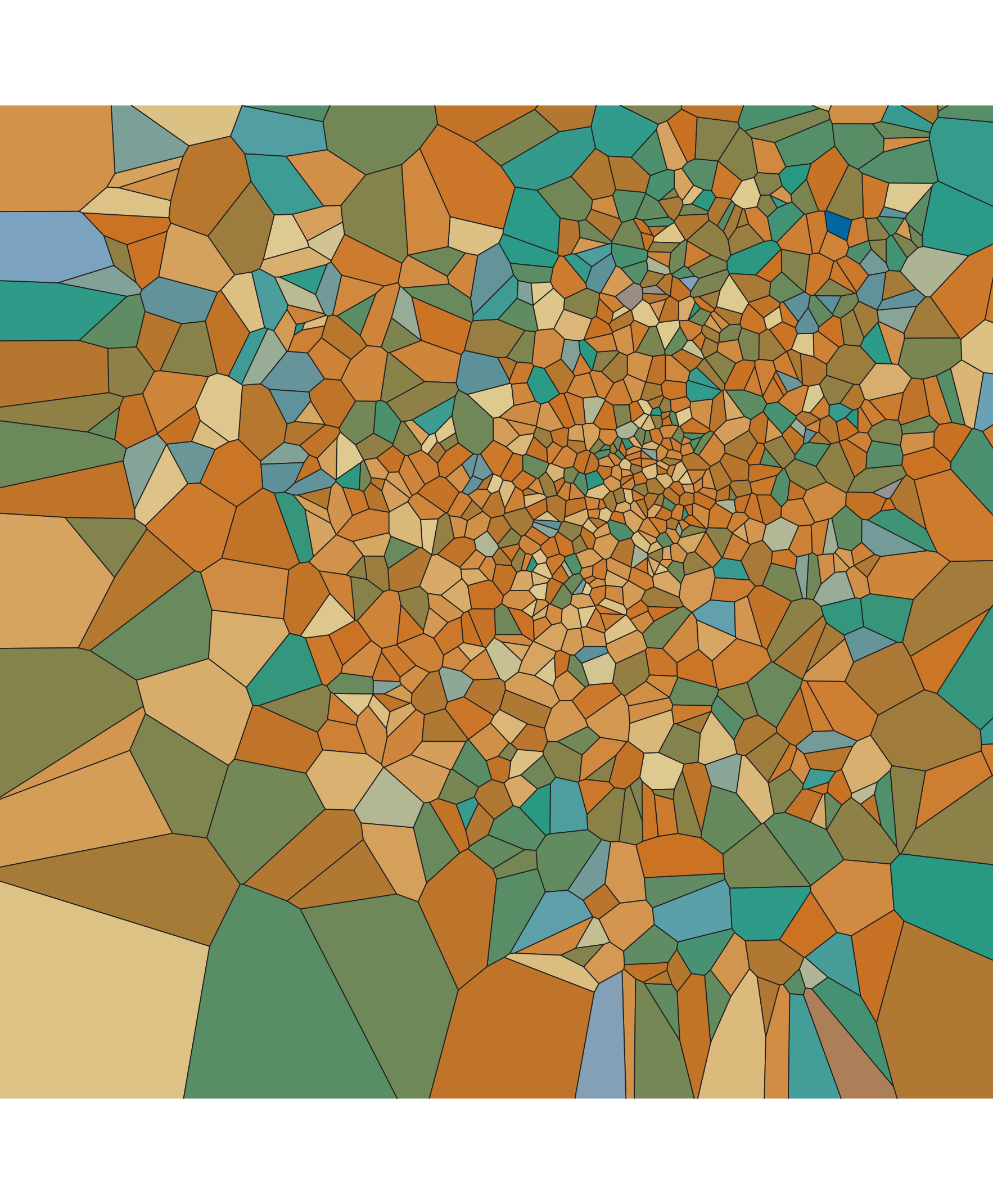
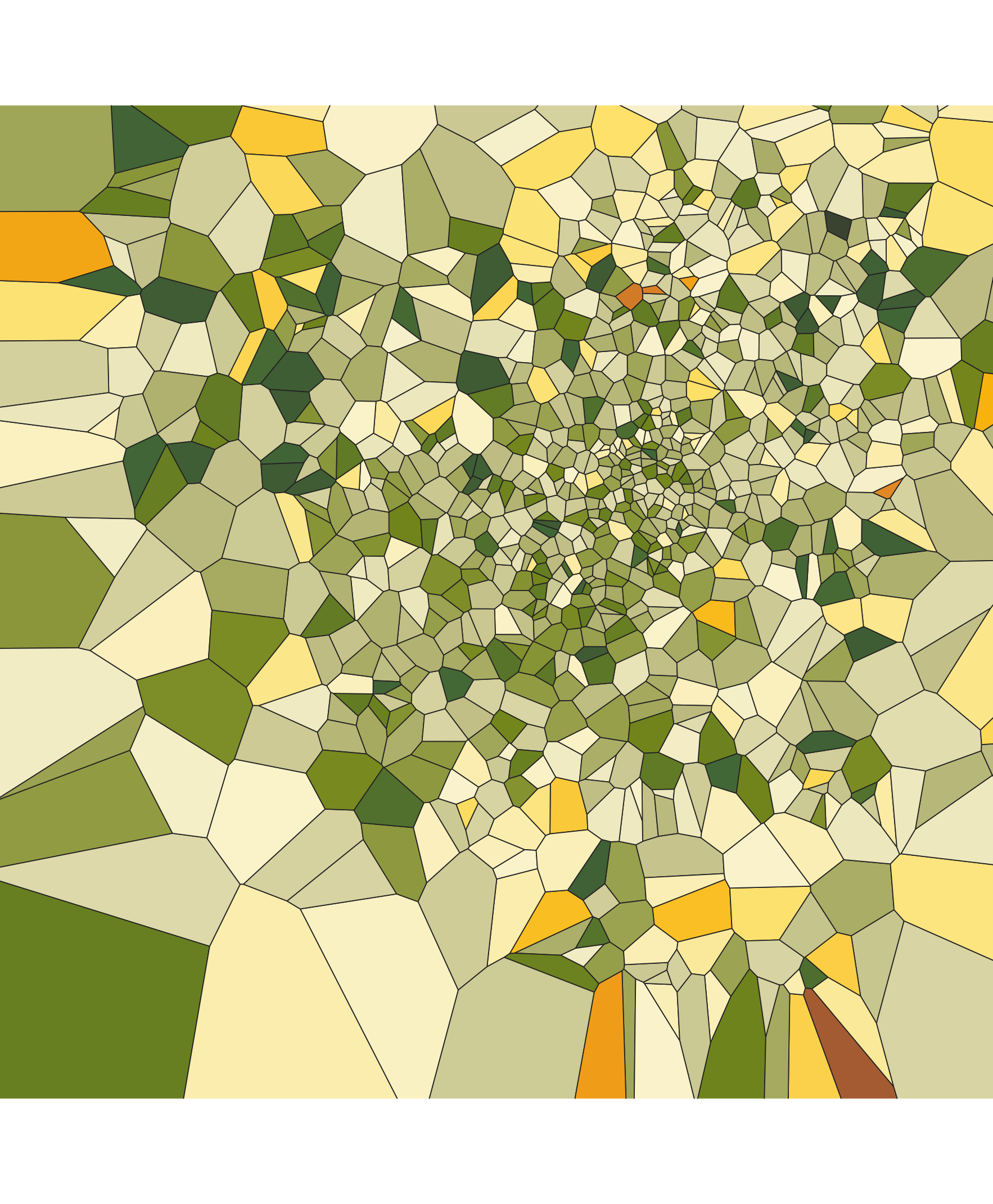
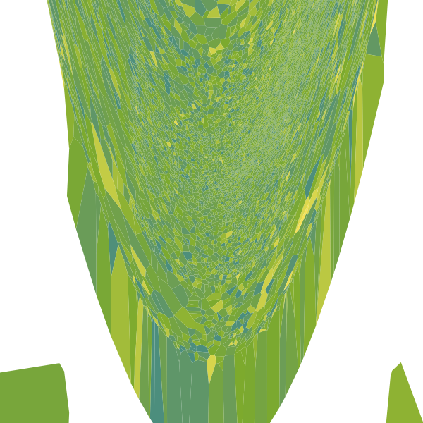
Whole unboxy grid but with different colors from sample_canva2():

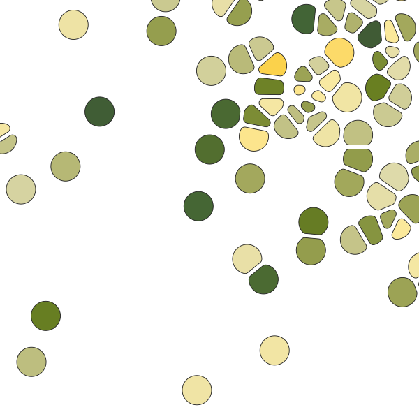
Goal: make 3 different plots based on different areas of the unboxy grid:

Studies in Voronoi baroque: Part II

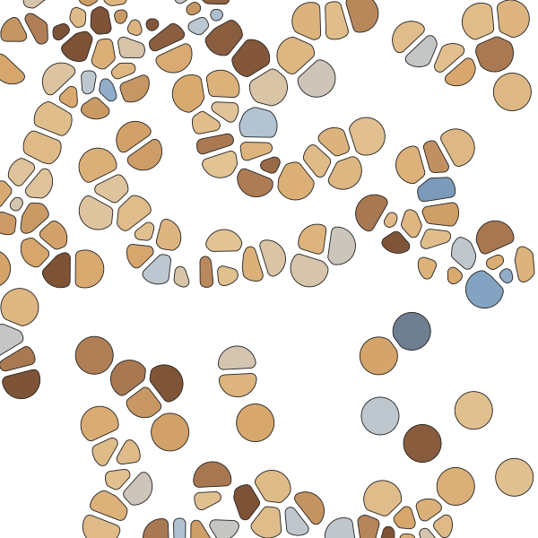
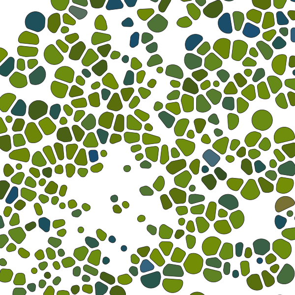
Functions:

Code

sift1 <- function(data) {
  data <- data |>
    group_by(group) |>
    mutate(
      tilesize = (max(x) - min(x)) * (max(y) - min(y)),
      x = if_else(tilesize > .02, x, x + rnorm(1)/10), 
      y = if_else(tilesize > .02, y, y + rnorm(1)/10)
    ) |>
    ungroup()
  return(data)
}

sift2 <- function(data) {
  data <- data |>
    group_by(group) |>
    mutate(
      tilesize = (max(x) - min(x)) * (max(y) - min(y)),
      # replacing tilesize arguments
      x = if_else(tilesize > 0.001, x, x + rnorm(1)), 
      y = if_else(tilesize > 0.001, y, y + rnorm(1, mean = 2, sd = 1))
    ) |>
    ungroup()
  return(data)
}

sift3 <- function(data) {
  data <- data |>
    group_by(group) |>
    mutate(
      tilesize = (max(x) - min(x)) * (max(y) - min(y)),
      x = if_else(tilesize > 1, x, x), 
      y = if_else(tilesize > 1, y, y + x^2)
    ) |>
    ungroup()
  return(data)
}

voronoi_baroque <- function(
    seed, 
    perturb, 
    max.radius = NULL, 
    radius = 0, 
    expand = 0,
    ...
) {
  
  set.seed(seed)
  
  blank <- ggplot(mapping = aes(x, y, fill = val)) +
    theme_void() + 
    coord_equal(xlim = c(-2.75, 2.75), ylim = c(-2.75, 2.75)) + 
    guides(fill = guide_none(), alpha = guide_none()) +
    scale_fill_gradientn(colours = sample_canva2(seed)) + 
    scale_alpha_identity() + 
    scale_x_continuous(expand = c(0, 0)) +
    scale_y_continuous(expand = c(0, 0))
  
  blank + 
    geom_voronoise(
      data = unboxy(iterations = 10000, layers = 5),
      perturb = perturb,
      max.radius = max.radius,
      radius = radius,
      expand = expand,
      ...,
      show.legend = FALSE
    )
}

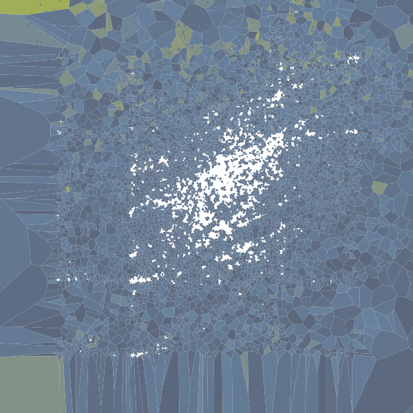
Playing around:

Code

voronoi1 <- voronoi_baroque(4564, sift1)
voronoi2 <- voronoi_baroque(5646, sift2)
voronoi3 <- voronoi_baroque(3243, sift3)

save(voronoi1, version = "01", width = 4, height = 4)
save(voronoi2, version = "01", width = 4, height = 4)
save(voronoi3, version = "01", width = 4, height = 4)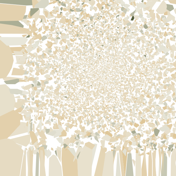

Truchet tiles

Example:

Code

set.seed(123)
mosaic <- st_truchet_ms(
  tiles = c("dr", "tn", "ane"), 
  p1 = 0.2, # scale 1 
  p2 = 0.6, # scale 2
  p3 = 0.2, # scale 3
  xlim = c(1, 6),
  ylim = c(1, 6)
)
mosaic %>% 
  ggplot(aes(fill = color)) +
  geom_sf(color = NA, show.legend = FALSE) + 
  scale_fill_gradientn(colours = c("#222222", "#ffffff")) + 
  theme_void()

set.seed(123)
st_truchet_ss(
  tiles = c(
    "silk_1", "silk_2", 
    "rainbow_1", "rainbow_2",
    "cloud_1", "cloud_2"
  ),
  xlim = c(1, 9),
  ylim = c(1, 6)
) |>
  ggplot() +
  geom_sf(colour = "white") +
  scale_x_continuous(expand = c(0, 0)) +
  scale_y_continuous(expand = c(0, 0)) +
  theme_void()

Playing around:

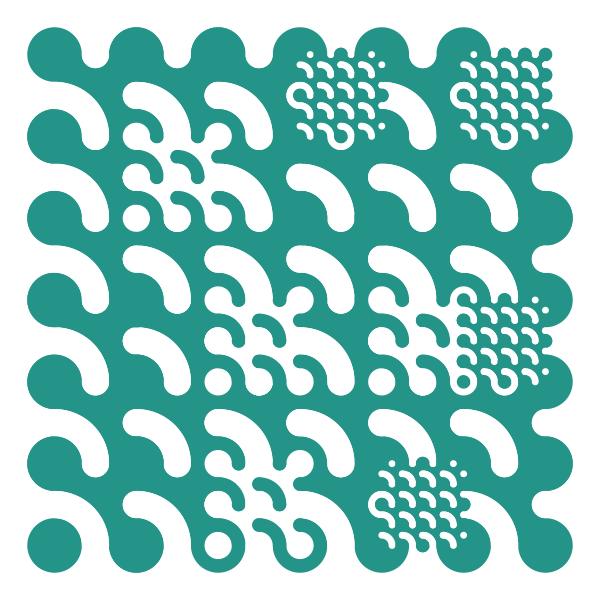
Tile types: ‘dl’,‘dr’,‘-’,‘|’,‘+.’,‘+’,‘x.’,‘tn’,‘fnw’,‘fne’,‘fsw’,‘fse’,‘ane’,‘asw’

Code

# test round 1 ----
mosaic1 <- st_truchet_ms(
  tiles = c("fsw"), 
  p1 = 0.8, # scale 1 
  p2 = 0.1, # scale 2
  p3 = 0.1, # scale 3
  xlim = c(1, 6),
  ylim = c(1, 6)
)

truchet1 <- mosaic1 %>% 
  ggplot(aes(fill = color)) +
  geom_sf(color = NA, show.legend = FALSE) + 
  scale_fill_gradientn(colours = c("#239487", "#ffffff")) + 
  theme_void()


# test round 2 ----
mosaic2 <- st_truchet_ms(
  tiles = c("+.", "|", "-", "x."), 
  p1 = 0.3, # scale 1 
  p2 = 0.5, # scale 2
  p3 = 0.2, # scale 3
  xlim = c(1, 6),
  ylim = c(1, 6)
) %>% 
  mutate(color2 = round(runif(length(color), min = 1, max = 5)))

truchet2 <- mosaic2 %>% 
  ggplot(aes(fill = color2)) +
  geom_sf(color = NA, show.legend = FALSE) + 
  scale_fill_gradientn(colours = natparks.pals("Olympic")) + 
  theme_void()

# test round 3 ----
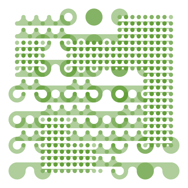
mosaic3 <- st_truchet_ms(
  tiles = c("tn"), 
  p1 = 0.33, # scale 1 
  p2 = 0.33, # scale 2
  p3 = 0.33, # scale 3
  xlim = c(1, 6),
  ylim = c(1, 6)
)

truchet3 <- mosaic3 %>% 
  ggplot(aes(fill = color)) +
  geom_sf(color = NA, show.legend = FALSE) + 
  scale_fill_gradientn(colors = c("#58972A78", "#FFFFFF")) +
  theme_void()

# test round 4 ----
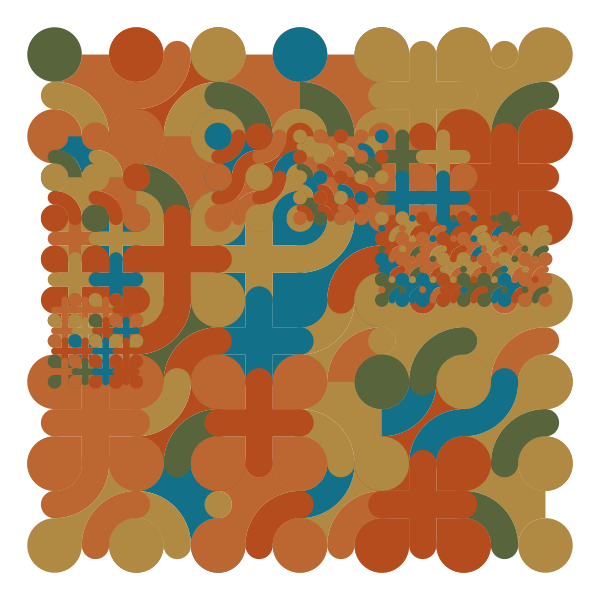
mosaic4 <- st_truchet_ms(
  tiles = c("asw", "dr", "+", "fse"), 
  p1 = 0.8, # scale 1 
  p2 = 0.1, # scale 2
  p3 = 0.1, # scale 3
  xlim = c(1, 6),
  ylim = c(1, 6)
) %>% 
  mutate(color2 = round(runif(length(color), min = 1, max = 5)))

truchet4 <- mosaic4 %>% 
  ggplot(aes(fill = color2)) +
  geom_sf(color = NA, show.legend = FALSE) + 
  scale_fill_gradientn(colours = natparks.pals("Saguaro")) + 
  theme_void()

# test round 5 ----
mosaic5 <- st_truchet_ms(
  tiles = c("fnw", "|", "ane", "x."), 
  p1 = 0.5, # scale 1 
  p2 = 0.3, # scale 2
  p3 = 0.2, # scale 3
  xlim = c(1, 6),
  ylim = c(1, 6)
)

truchet5 <- mosaic5 %>% 
  ggplot(aes(fill = color)) +
  geom_sf(color = NA, show.legend = FALSE) + 
  scale_fill_gradientn(colors = c("#A23479", "#FFFFFF")) +
  theme_void()

# test round 6 ----
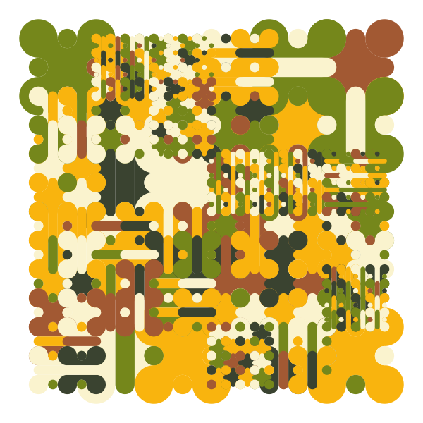
mosaic6 <- st_truchet_ms(
  tiles = c("-", "fnw", "x."), 
  p1 = 0.2, # scale 1 
  p2 = 0.2, # scale 2
  p3 = 0.6, # scale 3
  xlim = c(1, 6),
  ylim = c(1, 6)
) %>% 
  mutate(color2 = round(runif(length(color), min = 1, max = 10)))

truchet6 <- mosaic6 %>% 
  ggplot(aes(fill = color2)) +
  geom_sf(color = NA, show.legend = FALSE) + 
  # scale_fill_gradientn(colors = c("#489A87", "#FFFFFF")) +
  scale_fill_gradientn(colours = natparks.pals("Glacier", n = 10, type = "continuous")) + 
  theme_void()

Printing and saving:

Code

truchet1
truchet2
truchet3
truchet4
truchet5
truchet6

save(truchet1, version = "01", width = 4, height = 4)
save(truchet2, version = "01", width = 4, height = 4)
save(truchet3, version = "01", width = 4, height = 4)
save(truchet4, version = "01", width = 4, height = 4)
save(truchet5, version = "01", width = 4, height = 4)
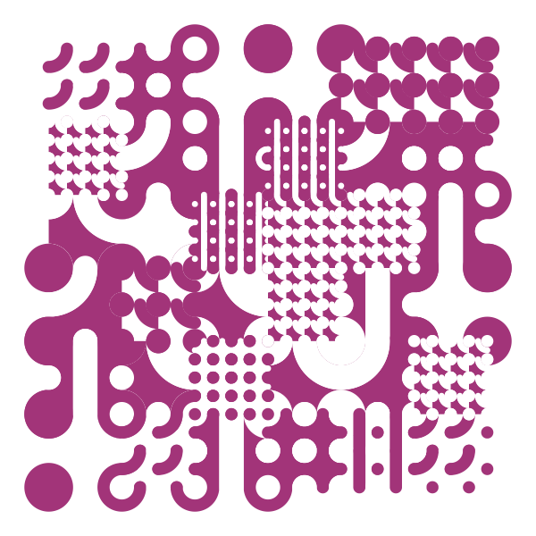
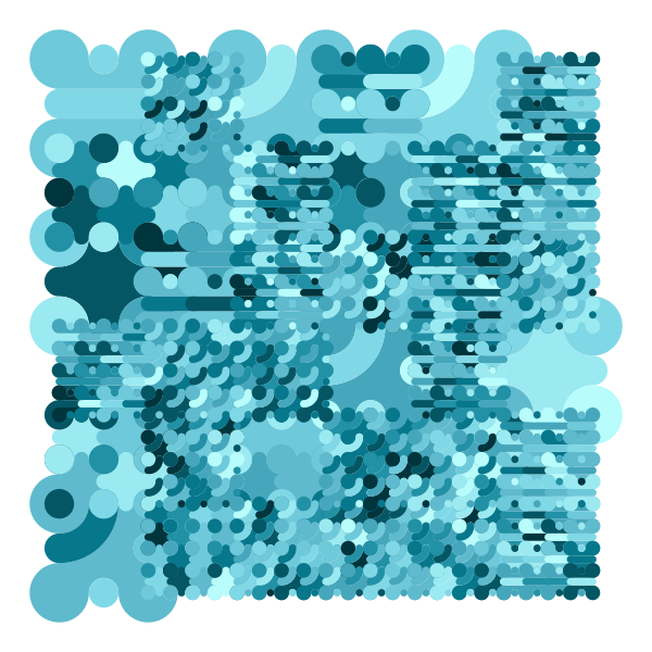
save(truchet6, version = "01", width = 4, height = 4)