2  Computing indices of biodiversity

Now that we have N from our previous model (or \(z\) or \(\psi\) for an occupancy model), we can calculate metrics of biodiversity. These can include any metric commonly used to describe \(\alpha\) or \(\beta\) diversity and can include taxonomic, phylogenetic, and functional diversity metrics.

Abundance-based metrics common in community ecology include Shannon diversity (taxonomic \(\alpha\) diversity), Bray-Curtis dissimilarity (taxonomic \(beta\) diversity), and Rao’s quadratic entropy (functional \(\alpha\) diversity). These can be derived from estimates of \(N\) from a MSAM or from estimates of \(\psi\) from an occupancy model (as pseudo-abundance data).

Occurrence-based metrics common in community ecology include species richness (taxonomic \(alpha\) diversity), Jaccard dissimilarity (taxonomic \(beta\) diversity), and functional richness (functional \(\alpha\) diversity). These can be derived from estimates of \(z\) from an occupancy model, or from data simplifed from an MSAM to describe presence-absence as opposed to abundance data.

Useful resources for biodiversity metrics and implementing them in R:(Oksanen et al. (2020); Hallett et al. (2016); Morris et al. (2014); Grenié and Gruson (2025))

We provide examples of many of these in the main text and supporting information of our paper. Further, these can be generated as derived quantities within a Bayesian model or using posterior samples of the above quantities (\(N\), \(z\), or \(\psi\)) in R.

2.1 Computing indices of biodiversity

2.1.1 Bray-Curtis Dissimilarity

Bray-Curtis dissimilarlity describes changes in overall community abundance across time or space. This index is calculated by breaking the two communities being compared into three parts:

1. The total number of shared individuals in communities 1 and 2 (A)
2. The total number of individuals in only community 1 (B)
3. The total number of individuals in only community 2 (C)

Then, dissimilarlity is calcluated as:

\(BC = \frac{(B + C)}{(2A + B + C)}\)

2.1.2 Species turnover

Species turnover is similar to Bray-Curtis dissimilarity - we break the two communities into three different groups:

1. The species shared between community 1 and 2 (A)
2. The species only in community 1 (B)
3. The species only in community 2 (C)

Then, turnover is:

\(turnover = \frac{(B + C)}{(A + B + C)}\)

For this study (plant dataset), we decomposed turnover into “gains” and “losses” by just including either \(B\) (losses) or \(C\) (gains) in the denominator.

2.1.3 Interpretting both metrics

In both metrics, values closer to 1 indicate that the two communities are more different (a larger fraction of individuals or species are different between communities 1 and 2 than are shared). In our case, we are calculating these change metrics between a given survey unit in a dataset (“community”) between adjacent timepoints. For most datasets, this means we are comparing communities in time y to time y+1. However, for one dataset (PFNP plants), survey intervals were > 1 year apart, so we compared communities between adjacent time points (e.g. 2007 and 2014, 2014 and 2021).

2.1.4 Notation in our paper

In the paper, we define a general biodiversity metric as \(d_{t,y}\). And use the mean (\(\bar{d}_{t,y}\)) and variance (\(Var(\bar{d}_{t,y})\)) of this value as “data” in the environmental regression model.

2.2 Biodiversity metrics in JAGS models

2.2.1 Model code

We can include these metrics as “derived quantities” in our MSAM models that we can pull from models after they have converged. You can also derive these quantities in R, and we provide an example in the code in the tutorial folder.

When incorporating derived quantities into JAGS code, these quantities come at the end of the model code that we highlighted in the previous step (“Accounting for imperfect detection”), but we do not provide the whole model here for brevity. To see the model with both components, you can look at our model file in the imperfect detection tutorial folder.

model{
  
  #...
  #This is all the model code that we provided in the 
  # "Accounting for Imperfect Detection" tab, so we do not provide it here, 
  #for brevity.
  
  #DERIVED QUANTIIES
  
  #Bray-Curtis dissimilarity
  for(t in 1:n.transects){
    for(y in (n.start[t]+1):n.end[t]){
      for(s in 1:n.species){
        # num individuals in both time periods per species
        a[s,t,y] <- min(N[s,t,y-1], N[s,t,y])
        # num individuals only in first time point
        b[s,t,y] <- N[s,t,y-1] - a[s,t,y]
        # num individuals only in second time point
        c[s,t,y] <- N[s,t,y] - a[s,t,y]
      }
      #for all years 2 onward:
      #total number of shared individuals across time periods
      A[t,y] <- sum(a[,t,y])
      #total number of individuals in only first time period
      B[t,y] <- sum(b[,t,y])
      #total number of individuals in only second time period
      C[t,y] <- sum(c[,t,y])
      
      #total bray-curtis (B+C)/(2A+B+C)
      num[t,y] <- B[t,y] + C[t,y]
      denom1[t,y] <- 2*A[t,y]+B[t,y]+C[t,y]
      #if all values are zero - this just keeps the eqn. from
      #dividing by zero
      denom[t,y] <- ifelse(denom1[t,y]==0,1, denom1[t,y])
      
      #Calculate Bray-Curtis dissimiarlity
      bray[t,y] <- num[t,y]/denom[t,y]
      
    }
  }
}

2.2.2 Updating the model to get biodiversity metrics

We updated our converged model for a short number of iterations to get good estimates of mean and standard deviation values for our biodiversity metrics. We then exported the mean and standard deviations for these metrics as “data” to be provided in the next model (Evaluating biodiversity in relation to environmental variables)

# Load packages -----------------------------------------------------------

package.list <- c("tidyverse", 'here', #general packages
                  'jagsUI') #jags wrapper

## Installing them if they aren't already on the computer
new.packages <- package.list[!(package.list %in% installed.packages()[,"Package"])]
if(length(new.packages)) install.packages(new.packages)

## And loading them
for(i in package.list){library(i, character.only = T)}

# Load converged model -----------------------------------------------------------

model <- readRDS(here('tutorials',
                      "01_imperfect_detect",
                      'data',
                      'model_outputs',
                      'MSAM_model_output.RDS'))

# Update model to track Bray-Curtis ------------------------------------------------

#now the parameter we want is just bray, none of the others
params2 <- c("bray")

#run this model so we have ~4000 samples to calculate mean and SD
model2 <- update(model,
                 parameters.to.save = params2,
                 n.iter = 1335,
                 parallel = TRUE)

# Extract summary stats of bray ------------------------------------------------

#get a summary of this model and the parameters we saved (bray)
sum <- summary(model2$samples)

#pull out mean and SD values from that summary
stats <- as.data.frame(sum$statistics) %>%
  rownames_to_column(var = 'parm') %>%
  filter(parm != "deviance") %>%
  #re-connect these values with their transect and year IDs
  separate(parm, 
           into = c("transect", "year"),
           sep = ",") %>%
  mutate(transect = str_sub(transect, 6, (nchar(transect))),
         year = str_sub(year, 1, (nchar(year)-1))) %>%
  mutate(transect = as.numeric(transect),
         year = as.numeric(year)) %>%
  #select only the variables of interest
  dplyr::select(transect, year, Mean, SD)

We have saved this dataframe in the imperfect detection tutorial folder.

Now we have a nice dataframe with mean (\(\bar{d}_{t,y}\)) and standard deviation (\(\hat{\sigma}(\bar{d}_{t,y})\)) for the Bray-Curtis dissimilarity calculated for each site along its time series. You will notice that the year value starts with year 2 and this is because this is the first year in which we have two community values to compare. and variance

str(stats)

'data.frame':   12 obs. of  4 variables:
 $ transect: num  1 2 3 1 2 3 1 2 3 1 ...
 $ year    : num  2 2 2 3 3 3 4 4 4 5 ...
 $ Mean    : num  0.664 0.638 0.616 0.486 0.505 ...
 $ SD      : num  0.0266 0.026 0.0252 0.0362 0.0372 ...

We can also look at how Bray-Curtis dissimilarity changes through time for each of our transects in our simulated datasets.

labels <- c("Transect 1", "Transect 2", "Transect 3")
names(labels) <- c('1', '2', '3')

ggplot(stats) +
  geom_ribbon(aes(x = year, ymin = Mean-SD, ymax = Mean+SD), alpha = 0.6) +
  geom_line(aes(x = year, y = Mean)) +
  facet_grid(~transect, labeller = labeller(transect = labels)) +
  theme_bw() +
  theme(strip.background = element_rect(fill = "white")) +
  labs(x = "Year", y = "Bray-Curtis dissimilarity \n (Posterior mean and SD)")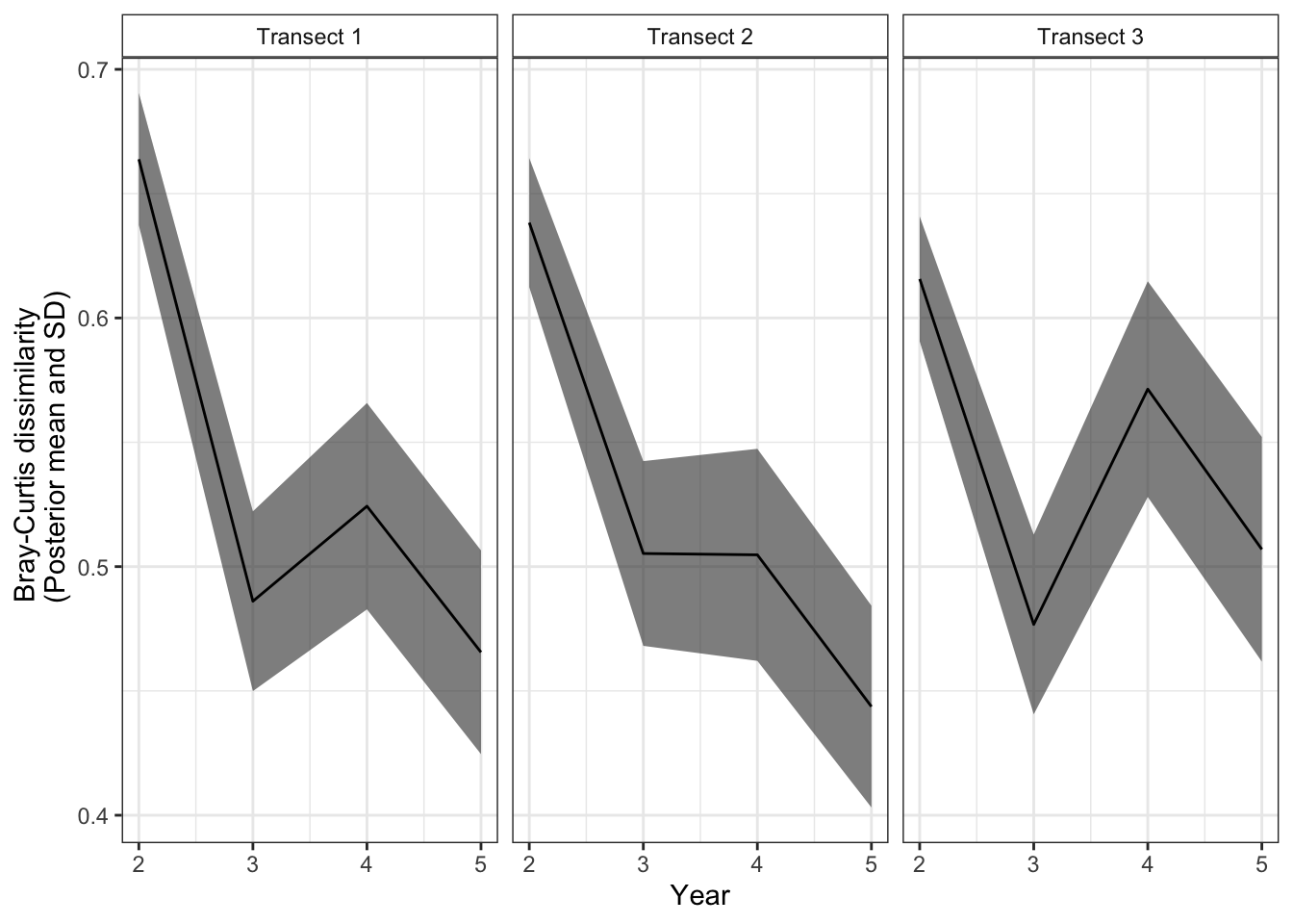

2.2.3 Next: Evaluating biodiversity in relation to environmental variables

Next we will take the mean and standard deviation of these biodiversity values and incorporate them into a regression with environmental covariates to examine how these covariates shape communities.

Grenié, M, and H Gruson. 2025. Fundiversity: Easy Computation of Functional Diversity Indices. https://CRAN.R-project.org/package=fundiversity.

Hallett, Lauren M., Sydney K. Jones, A. Andrew M. MacDonald, Matthew B. Jones, Dan F. B. Flynn, Julie Ripplinger, Peter Slaughter, Corinna Gries, and Scott L. Collins. 2016. “Codyn: Anrpackage of Community Dynamics Metrics.” Edited by Timothée Poisot. Methods in Ecology and Evolution 7 (10): 1146–51. https://doi.org/10.1111/2041-210x.12569.

Morris, E. Kathryn, Tancredi Caruso, François Buscot, Markus Fischer, Christine Hancock, Tanja S. Maier, Torsten Meiners, et al. 2014. “Choosing and Using Diversity Indices: Insights for Ecological Applications from the German Biodiversity Exploratories.” Ecology and Evolution 4 (18): 3514–24. https://doi.org/10.1002/ece3.1155.

Oksanen, Jari, F. Guillaume Blanchet, Michael Friendly, Roeland Kindt, Pierre Legendre, Dan McGlinn, Peter R. Minchin, et al. 2020. Vegan: Community Ecology Package. https://CRAN.R-project.org/package=vegan.