3  Evaluating biodiversity in relation to environmental variables

We have used our estimates of detection error to correct our values of biodiversity. Now, we are interested in how biodiversity is influenced by environmental covariates at our site. However, in doing so, we also want to maintain both the mean estimate value as well as uncertainty estimated by the imperfect detection modeling process, so we will have to provide this in our model structure.

3.1 Model formulation

Like many diversity metrics, our diversity metrics are functionally proportions, so the data have domain \([0,1]\). We can model proportions with a beta distribution, where the mean metric calculated in the previous step, \(\bar{d}_{t,y}\), is beta distributed:

\(\bar{d}_{t,y} \sim Beta(\alpha_{t,y}, \beta_{t,y})\)

We follow other beta regression approaches (Irvine, Rodhouse, and Keren (2016); Ferrari and Cribari-Neto (2004)) to define the parameters \(\alpha_{t,y}\) and \(\beta_{t,y}\) as:

\(\alpha_{t,y} = \delta_{t,y}\phi_{t,y}\)

\(\beta_{t,y} = (1 - \delta_{t,y})\phi_{t,y}\)

In these equations, \(\delta_{t,y}\) is the mean or expected value of the biodiversity index, \(\bar{d}_{t,y}\) and \(\phi_{t,y}\) is a precision-type term. When \(\phi_{t,y}\) is larger, the variance for \(\bar{d}_{t,y}\) (\(Var(\bar{d}_{t,y})\)) is smaller. \(\phi_{t,y}\) is defined as:

\(\phi_{t,y} = \frac{\delta_{t,y}(1-\delta_{t,y})}{Var(\bar{d}_{t,y})}-1\)

and \(Var(\bar{d}_{t,y})\) includes both known variance from the imperfect detection model, \(\hat{\sigma}^2(\bar{d}_{t,y})\), and unknown “process” variance, \(\sigma^2_{P}\):

\(Var(\bar{d}_{t,y}) = \hat{\sigma}^2(\bar{d}_{t,y}) + \sigma^2_{P}\)

We set a uniform prior for the process variance, \(\sigma^2_{P}\) with an upper limit that ensures that \(\alpha_{t,y} > 0\) and \(\beta_{t,y} > 0\).

The mean (expected) biodiversity index, \(\delta_{t,y}\), is defined via a regression model:

\(logit(\delta_{t,y}) = \beta_{0,t} + \sum_{j =1}^J\beta_jZ_{j,t,y}\)

In this regression, \(\beta_{0,t}\) varies by a spatial factor by including a spatial random effect with priors that are hierarchically centered around a coarser spatial level, which is given a prior that varies around an overall community intercept (Ogle and Barber 2020). The coefficients \(\beta_1\), \(\beta_2\)… \(\beta_J\) denote the effects of an antecedent covariate, \(Z_{j,t,y}\) for j = 1, 2, …,J covariates. Each covariate \(Z_{j,t,y}\) is the weighted average of the current value for that covariate at time y and a defined number of past values for that covariate preceding time y. We divided these into either seasonal or yearly values for that covariate (e.g., spring temperature, yearly plant biomass). The weight (“importance weight”) of each of these values, m, in the overall calculation of \(Z_{j,t,y}\), \(w_{j,m}\), is estimated by the model using the stochastic antecedent modeling framework (Ogle et al. 2015). In this modeling framework, each \(w_{j,m}\) is estimated using a Dirichlet prior so that the sum across all weights for that covariate equals one and more important time periods, m get higher importance weights. Thus, when a covariate effect, \(\beta_j\) is significant, the weights for each time lag for that covariate informs over which timescale(s) that covariate influences biodiversity.

While the process will be different for some biodiversity metrics (e.g., species richness, Shannon diversity), similar partitioning of variance can be performed for other data distributions (e.g., Poisson) by using the mean \(E(x)\) and variance \(Var(x)\) equations for any distribution.

3.1.1 The model translated to JAGS code

Below is example JAGS code for the model specified above:

model{
  
  for(i in 1:n.data){
    
    #-------------------------------------## 
    # Likelihood ###
    #-------------------------------------##
    
    #d is dissimilarity and is proportional, so beta distribution works here
    d[i] ~ dbeta(alpha[i], beta[i])
      
    #var.process is scalar but could be made dependent on site/other variables
    #phi incorporates mu (mean estimate), var.estimate (which is from
    #"data" on standard deviation (squared) from the original detection 
    #correction model) 
    #and var.process is something we're trying to estimate,
    #basically, the rest of the variation not accounted for
    phi[i] <- (((1-mu[i])*mu[i])/(var.estimate[i] + var.process))-1

    #alpha and beta are based on mu and phi values
    #sometimes these values send alpha and beta outside
    #the domain, so we have extra code below to get them to
    #stay where they belong
    alphaX[i] <- mu[i] * phi[i]
    betaX[i] <- (1 - mu[i]) * phi[i]
    
    #here is where we get alpha and beta to stay in their
    #domain
    alpha[i] <- max(0.01, alphaX[i])
    beta[i] <- max(0.01, betaX[i])
    
    #to get a good estimate of a prior for var.process, we
    #track the difference between these two values for each
    #data point
    diff[i] <- (1-mu[i])*mu[i] - var.estimate[i]

    #Regression of mu, which is dependent on a hierrarchically-centered
    #site random effect and the weighted antecedent effects of two covariates,
    #plant biomass and temperature
      logit(mu[i]) <- b0.site[Site.ID[i]] +
        b[1]*AntCov1[i] +
        b[2]*AntCov2[i]
      
      #-------------------------------------## 
      # SAM summing ###
      #-------------------------------------##
      
      #summing the antecedent values
      AntCov1[i] <- sum(Cov1Temp[i,]) #summing across the total number of antecedent years
      AntCov2[i] <- sum(Cov2Temp[i,]) #summing across the total num of antecedent months

      #Generating each year's weight to sum above
      for(t in 1:n.lag1){ #number of time steps we're going back in the past
        Cov1Temp[i,t] <- Cov1[i,t]*wA[t] 
      
        #imputing missing data
        Cov1[i,t] ~ dnorm(mu.cov1, tau.cov1)
      }
        
      #generating each month's weight to sum above
      for(t in 1:n.lag2){ #number of time steps we're going back in the past
        Cov2Temp[i,t] <- Cov2[i,t]*wB[t] 

        #missing data
        Cov2[i,t] ~ dnorm(mu.cov2, tau.cov2)
      }
      
      #-------------------------------------## 
      # Goodness of fit parameters ###
      #-------------------------------------##
      # 
      #replicated data
      d.rep[i] ~ dbeta(alpha[i], beta[i])
      # 
      #residuals
      resid[i] <- d[i] - mu[i]
 
  }
  
  #-------------------------------------## 
  # Priors ###
  #-------------------------------------##
  
  # ANTECEDENT CLIMATE PRIORS
  #Sum of the weights for lag
  sumA <- sum(deltaA[]) #all the plant weights
  
  #Employing "delta trick" to give vector of weights dirichlet priors
  #this is doing the dirichlet in two steps 
  #see Ogle et al. 2015 SAM model paper in Ecology Letters
  for(t in 1:n.lag1){ #for the total number of lags
    #the weights for kelp - getting the weights to sum to 1
    wA[t] <- deltaA[t]/sumA
    #and follow a relatively uninformative gamma prior
    deltaA[t] ~ dgamma(1,1)
    
    #to look at how weights accumulate through time
    cumm.wt1[t] <- sum(wA[1:t])
  }
  
  #Sum of the weights for temp lag
  sumB <- sum(deltaB[]) #all the temp weights
  
  #Employing "delta trick" to give vector of weights dirichlet priors
  #this is doing the dirichlet in two steps 
  #see Ogle et al. 2015 SAM model paper in Ecology Letters
  for(t in 1:n.lag2){ #for the total number of lags
    #the weights for kelp - getting the weights to sum to 1
    wB[t] <- deltaB[t]/sumB
    #and follow a relatively uninformative gamma prior
    deltaB[t] ~ dgamma(1,1)
    
    #to look at cummulative weigths through time
    cumm.wt2[t] <- sum(wB[1:t])
  }
  
  #BETA PRIORS
  #HIERARCHICAL STRUCTURE PRIORS
  #hierarchical centering of sites on b0
   for(s in 1:n.sites){
     b0.site[s] ~ dnorm(b0, tau.site)
   }
  
  #overall intercept gets relatively uninformative prior
  b0 ~ dnorm(0, 1E-2)
  
  #for low # of levels, from Gelman paper - define sigma
  # as uniform and then precision in relation to this sigma
  sig.site ~ dunif(0, 10)
  tau.site <- 1/pow(sig.site,2)
  
  #covariate effects - again get relatively uninformative priors
  for(i in 1:2){
    b[i] ~ dnorm(0, 1E-2)
  }
  
  #PRior for process error
  var.process ~ dunif(0, min(diff[]))


  #MISSING DATA PRIORS
  mu.cov1 ~ dunif(-10, 10)
  sig.cov1 ~ dunif(0, 20)
  tau.cov1 <- pow(sig.cov1, -2)
  mu.cov2 ~ dunif(-10, 10)
  sig.cov2 ~ dunif(0, 20)
  tau.cov2 <- pow(sig.cov2, -2)
  
}

3.2 The model in action

Because we have greatly reduced the dimensionality of our community dataset by deriving a change metric for each site in each year, y to the next year y+1, the models run efficiently enough that we can use real data for this tutorial. We will demonstrate the utility of this model for the grasshopper dataset from Sevilleta LTER used in our examples in the paper. This LTER site also has high-resolution information for temperature, precipitation, and plant biomass.

This dataset has:

• 60 communities (survey transects) which have change data for
• 27 years, and we calculated
• Bray-Curtis dissimilarity for this count dataset
• 6 seasons of temperature and precipitation data and
• 11 seasons of plant data as covariates

In this dataset, we are evaluating how Bray-Curtis dissimilarity through time is shaped by the covariates of temperature, precipitation, and plant biomass.

Again, to run the model in R and JAGS, we will need:

• The model file
• The data list
• A script to wrap JAGS in R

You can find all of these, along with the tidy data and script used to prep the data list for this example, in the beta regression tutorial folder

3.2.1 Running the model

3.2.1.1 The model file

You will need to provide a path to the model file (which is its own R script, written in JAGS/BUGS language, so it won’t actually run in R). You can find ours here. You will see that we define the path to this model in our model running script below.

3.2.1.2 The data list

To run the model, we will need to provide JAGS with a data list, which you can find here. We have code on how to prepare the data list here.

data_list <- readRDS(here('tutorials',
                          '03_beta_regression',
                          'data',
                          "model_inputs",
                          "grasshopper_betareg_input_data_list.RDS"))

str(data_list)

List of 13
 $ n.data      : int 1260
 $ n.webs      : int 10
 $ n.templag   : int 6
 $ n.npplag    : int 11
 $ n.pptlag    : int 6
 $ n.transects : int 60
 $ bray        : num [1:1260] 0.26 0.261 0.283 0.339 0.425 ...
 $ var.estimate: num [1:1260] 0.00234 0.00347 0.00221 0.00204 0.00278 ...
 $ Web.ID      : num [1:1260] 1 1 1 1 1 1 1 1 1 1 ...
 $ Transect.ID : int [1:1260] 1 1 1 1 1 1 1 1 1 1 ...
 $ Temp        : num [1:1260, 1:6] -0.845 -1.009 -1.06 -1.031 -0.971 ...
  ..- attr(*, "dimnames")=List of 2
  .. ..$ : NULL
  .. ..$ : chr [1:6] "Temp" "Temp_l1" "Temp_l2" "Temp_l3" ...
 $ PPT         : num [1:1260, 1:6] 0.771 0.534 0.499 1.148 0.211 ...
  ..- attr(*, "dimnames")=List of 2
  .. ..$ : NULL
  .. ..$ : chr [1:6] "PPT" "PPT_l1" "PPT_l2" "PPT_l3" ...
 $ NPP         : num [1:1260, 1:11] -0.4807 -0.8532 -0.2417 0.0536 -0.8767 ...
  ..- attr(*, "dimnames")=List of 2
  .. ..$ : NULL
  .. ..$ : chr [1:11] "NPP" "NPP_l1" "NPP_l2" "NPP_l3" ...

As you can see, this data list includes indexing numbers, vectors, matrices, and arrays to pass to JAGS.

3.2.1.3 The script to run the model

Just like with the imperfect detection model, we’ll run the model using the jagsUI wrapper package. You can find this script here, and the general code to run a JAGS model is provided here:

# Load packages ---------------------------------------------------------------

# Load packages, here and tidyverse for coding ease, 
package.list <- c("here", "tidyverse", #general packages for data input/manipulation
                  "jagsUI", #to run JAGS models
                  'mcmcplots', #to look at trace plots
                  "coda",'patchwork') #to evaluate convergence
                   

## Installing them if they aren't already on the computer
new.packages <- package.list[!(package.list %in% 
                                 installed.packages()[,"Package"])]
if(length(new.packages)) install.packages(new.packages)

## And loading them
for(i in package.list){library(i, character.only = T)}


# Load data ---------------------------------------------------------------

data_list <- readRDS(here('tutorials',
                          '03_beta_regression',
                          'data',
                          "model_inputs",
                          "grasshopper_betareg_input_data_list.RDS"))


# Define model path -------------------------------------------------------

model <- here('tutorials',
              '03_beta_regression',
              'code',
              'grasshopper_betareg_model.R')

# Parameters to save ------------------------------------------------------

#these parameters we can track to assess convergence
params <- c('b0.web', #site-level intercepts
            'b0', #overall intercept
            'b', #covariate effects
            'wA', #plant biomass weights vector
            'wB', #temperature weights
            'sig.site', #sd of site effects
            'var.process') #unknown variance

# JAGS model --------------------------------------------------------------

mod <- jagsUI::jags(data = data_list,
                    inits = NULL,
                    model.file = model,
                    parameters.to.save = params,
                    parallel = TRUE,
                    n.chains = 3,
                    n.iter = 350,
                    DIC = TRUE)


# Check convergence -------------------------------------------------------
# 
mcmcplot(mod$samples)
# 
gelman.diag(mod$samples, multivariate = F)

Again, depending on your computer and/or datasets, you may need to re-run this model with initial values for root nodes and use cloud computing to run this model.

3.2.2 Model results

Once you have a resulting model file (which could be quite large), you can generate a summary of it:

sum <- summary(mod$samples)

This model requires some re-running with initial values, which we have done and provide a summary from the converged model in the tutorial folder. We can look at estimated values from this summary to assess how temperature, precipitation, and plant biomass impact grasshopper communities.

3.2.2.1 Covariate effects

theme_set(theme_bw())
#pull median and 95% BCI out of the summary file:
betas <- as.data.frame(sum$quantiles) %>%
  #get parameter names to be a column
    rownames_to_column(var = "parm") %>%
  #select only the covariate effect betas
    filter(str_detect(parm, "b")) %>%
    filter(!str_detect(parm, "b0")) %>%
  filter(!str_detect(parm, "web"))

#plot these median and 95% BCI values
ggplot(betas, aes(x = `50%`, y = parm)) +
  geom_vline(xintercept = 0, linetype = 2, alpha = 0.4) +
  geom_pointrange(aes(x = `50%`,
                      y = parm, 
                      xmin = `2.5%`,
                      xmax = `97.5%`),
                  size = 0.4) +
  scale_y_discrete(labels = c("Temperature", "Precipitation",
                              'Plant biomass')) + 
  labs(x = "Covariate effect \n (Median and 95% BCI)",
       y = "") +
  theme_bw()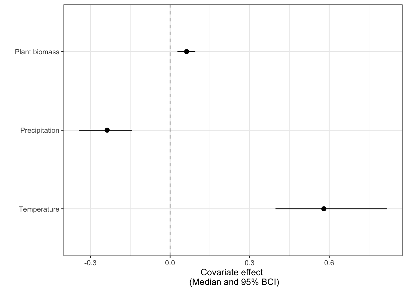

This figure suggests that there is a clear effect of all three covariates on Bray-Curtis dissimilarity. Higher temperatures and plant biomass lead to higher community change; higher precipitation leads to lower community change. We can then look at which seasons drive these effects:

#pull the median and 95% BCI weights for temperature out of the model summary file
hopper_weights <- as.data.frame(sum$quantiles) %>%
  rownames_to_column(var = "par") %>%
  filter(str_detect(par, "w")) %>%
  filter(!str_detect(par, "cumm")) %>%
  filter(!str_detect(par, "b0.web")) %>%
  filter(!str_detect(par, "sig.web")) %>%
  mutate(lag = str_sub(par, 4, (nchar(par)-1))) %>%
  mutate(covariate = case_when(str_detect(par, "wA") ~ "Temperature",
                               str_detect(par, "wB") ~ "Precipitation",
                               str_detect(par, "wC") ~ "Plant biomass")) %>%
  dplyr::select(lag, covariate, `2.5%`, `50%`, `97.5%`)

hop_weight_plot1 <- hopper_weights %>%
    filter(covariate == "Plant biomass") %>%
    mutate(lag = factor(lag, levels = c("1", "2", 
                                        "3", "4", "5",
                                        "6", "7", "8",
                                        "9", "10",
                                        "11"))) %>%
    ggplot(aes(x = lag, y = `50%`)) +
    geom_hline(yintercept = 1/11, linetype = 2, alpha = 0.4) +
    geom_pointrange(aes(x = lag, 
                        y = `50%`,
                        ymin = `2.5%`,
                        ymax = `97.5%`),
                    position=position_dodge(width=0.5),
                    size = 0.4) +
    facet_grid(~covariate)+
    labs(x= "Seasons into past",
         y = "Importance weight\n(median and 95% BCI)")

hop_weight_plot2 <- hopper_weights %>%
    filter(covariate != "Plant biomass") %>%
    mutate(lag = factor(lag, levels = c("1", "2", 
                                        "3", "4", "5",
                                        "6"))) %>%
    ggplot(aes(x = lag, y = `50%`)) +
    geom_hline(yintercept = 1/6, linetype = 2, alpha = 0.4) +
    geom_pointrange(aes(x = lag, 
                        y = `50%`,
                        ymin = `2.5%`,
                        ymax = `97.5%`),
                    position=position_dodge(width=0.5),
                    size = 0.4) +
    facet_grid(~covariate)+
    labs(x= "Seasons into past",
         y = "Importance weight\n(median and 95% BCI)") +
  theme(axis.title.y = element_blank())

hop_weight_plot1 +hop_weight_plot2 +
  plot_layout(widths = c(1.5,2))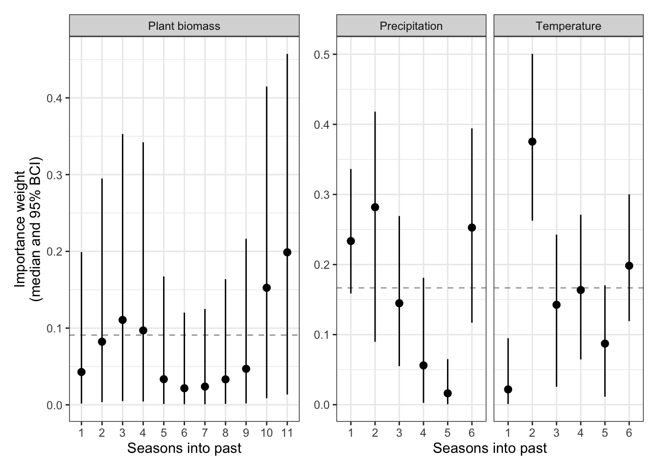

The dashed line indicates the values of importance weights if they were all equal (their prior weights). Any values clearly above this line indicate more important seasons. For plant biomass, we can see that there aren’t any clearly more important seasons, though some suggestion that more current seasons and seasons 2 years ago may be more important. For precipitation, it appears that this season is most important, but there may be a longer temporal signal if we added more time lags (when the current “wet” season is more wet, there is less community change). For temperature, last “warm” season (the season before the current one) is most important (when the previous warm season is warmer, there is more community change).

3.3 Wrapping up

For all models, you will want to be able to describe some kind of goodness-of-fit metric. We do this by replicating data in the model (e.g., d.rep in the model above) and then comparing the relationship between replicated data and observed data using a simple linear regression (Conn et al. 2018).

Conn, Paul B., Devin S. Johnson, Perry J. Williams, Sharon R. Melin, and Mevin B. Hooten. 2018. “A Guide to Bayesian Model Checking for Ecologists.” Ecological Monographs 88 (4): 526–42. https://doi.org/10.1002/ecm.1314.

Ferrari, Silvia, and Francisco Cribari-Neto. 2004. “Beta Regression for Modelling Rates and Proportions.” Journal of Applied Statistics 31 (7): 799–815. https://doi.org/10.1080/0266476042000214501.

Irvine, Kathryn M., T. J. Rodhouse, and Ilai N. Keren. 2016. “Extending Ordinal Regression with a Latent Zero-Augmented Beta Distribution.” Journal of Agricultural, Biological and Environmental Statistics 21 (4): 619–40. https://doi.org/10.1007/s13253-016-0265-2.

Ogle, Kiona, and Jarrett J. Barber. 2020. “Ensuring Identifiability in Hierarchical Mixed Effects Bayesian Models.” Ecological Applications 30 (7): e02159. https://doi.org/10.1002/eap.2159.

Ogle, Kiona, Jarrett J. Barber, Greg A. Barron-Gafford, Lisa Patrick Bentley, Jessica M. Young, Travis E. Huxman, Michael E. Loik, and David T. Tissue. 2015. “Quantifying Ecological Memory in Plant and Ecosystem Processes.” Edited by Elsa Cleland. Ecology Letters 18 (3): 221–35. https://doi.org/10.1111/ele.12399.